This page describes a method to generate polynomial trajectories that avoid passing through walls by solving a Quadratic Programming (QP) problem. 1D and 2D examples are provided with Python code. The paper describing this technique calls the free regions (non-wall area) Safe Flight Corridors (SFC) because each polynomial segment is surrounded by walls creating a polyhedron where the trajectory is allowed to pass. It is recommended to read QP Trajectory Generation before proceeding because this page builds on what was discussed there.
The first example is to generate a trajectory that minimizes snap and also passes through the following waypoints at the following times:
| i | t | x |
|---|---|---|
| 0 | 0 | 0 |
| 1 | 10 | 5 |
| 2 | 30 | 5 |
| 3 | 40 | 3 |
There is also a wall at x=5.5 and the position must not go above this value.
The QP problem has the form:
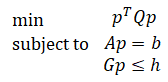
where p, Q, A, b are derived here. The problem now is to rewrite the wall constraint as an inequality and come up with G and h.
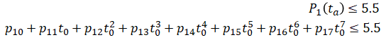
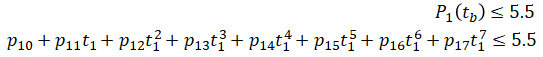
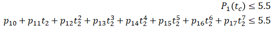
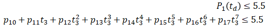
For simplicity, we will only consider the polynomial segment between waypoints 1 and 2 because that is where the trajectory curve overshoots and passes through the wall. We take four points between that segment:

where
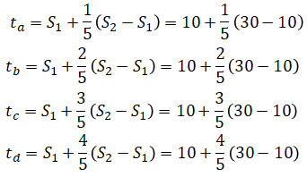
Let
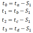
Then the constraints are:
which can be rewritten in Gp ≤ h form as,
Solving the QP:
import numpy as np
from cvxopt import matrix, solvers
import matplotlib.pyplot as plt

def get_Qi(T):
    return np.array([
        [0, 0, 0, 0, 0, 0, 0, 0],
        [0, 0, 0, 0, 0, 0, 0, 0],
        [0, 0, 0, 0, 0, 0, 0, 0],
        [0, 0, 0, 0, 0, 0, 0, 0],
        [0, 0, 0, 0, 1152*T, 2880*T**2, 5760*T**3, 10080*T**4],
        [0, 0, 0, 0, 2880*T**2, 9600*T**3, 21600*T**4, 40320*T**5],
        [0, 0, 0, 0, 5760*T**3, 21600*T**4, 51840*T**5, 100800*T**6],
        [0, 0, 0, 0, 10080*T**4, 40320*T**5, 100800*T**6, 201600*T**7]
    ])

def get_Q(T):
    Z = np.zeros((8, 8))
    Q0 = get_Qi(T[0])
    Q1 = get_Qi(T[1])
    Q2 = get_Qi(T[2])
    return np.block([
        [Q0, Z, Z],
        [Z, Q1, Z],
        [Z, Z, Q2]
    ])

def get_G(T):
    G = np.zeros((4, 8*3))
    G[0,8:16] = [1, T[1]/5, (T[1]/5)**2, (T[1]/5)**3, (T[1]/5)**4, (T[1]/5)**5, (T[1]/5)**6, (T[1]/5)**7]
    G[1,8:16] = [1, 2*T[1]/5, (2*T[1]/5)**2, (2*T[1]/5)**3, (2*T[1]/5)**4, (2*T[1]/5)**5, (2*T[1]/5)**6, (2*T[1]/5)**7]
    G[2,8:16] = [1, 3*T[1]/5, (3*T[1]/5)**2, (3*T[1]/5)**3, (3*T[1]/5)**4, (3*T[1]/5)**5, (3*T[1]/5)**6, (3*T[1]/5)**7]
    G[3,8:16] = [1, 4*T[1]/5, (4*T[1]/5)**2, (4*T[1]/5)**3, (4*T[1]/5)**4, (4*T[1]/5)**5, (4*T[1]/5)**6, (4*T[1]/5)**7]
    return G

def get_h(wall):
    return np.array([wall, wall, wall, wall])

def get_A(T):
    A = np.zeros((14, 8*3))
    # Start position of polynomials
    A[0,:8] = [1, 0, 0, 0, 0, 0, 0, 0]
    A[1,8:16] = [1, 0, 0, 0, 0, 0, 0, 0]
    A[2,16:] = [1, 0, 0, 0, 0, 0, 0, 0]
    # End position of polynomials
    A[3,:8] = [1, T[0], T[0]**2, T[0]**3, T[0]**4, T[0]**5, T[0]**6, T[0]**7]
    A[4,8:16] = [1, T[1], T[1]**2, T[1]**3, T[1]**4, T[1]**5, T[1]**6, T[1]**7]
    A[5,16:] = [1, T[2], T[2]**2, T[2]**3, T[2]**4, T[2]**5, T[2]**6, T[2]**7]
    # Continuous velocity
    A[6,:16] = [0, 1, 2*T[0], 3*T[0]**2, 4*T[0]**3, 5*T[0]**4, 6*T[0]**5, 7*T[0]**6, 0, -1, 0, 0, 0, 0, 0, 0]
    A[7,8:] = [0, 1, 2*T[1], 3*T[1]**2, 4*T[1]**3, 5*T[1]**4, 6*T[1]**5, 7*T[1]**6, 0, -1, 0, 0, 0, 0, 0, 0]
    # Continuous acceleration
    A[8,:16] = [0, 0, 2, 6*T[0], 12*T[0]**2, 20*T[0]**3, 30*T[0]**4, 42*T[0]**5, 0, 0, -2, 0, 0, 0, 0, 0]
    A[9,8:] = [0, 0, 2, 6*T[1], 12*T[1]**2, 20*T[1]**3, 30*T[1]**4, 42*T[1]**5, 0, 0, -2, 0, 0, 0, 0, 0]
    # Continuous jerk
    A[10,:16] = [0, 0, 0, 6, 24*T[0], 60*T[0]**2, 120*T[0]**3, 210*T[0]**4, 0, 0, 0, -6, 0, 0, 0, 0]
    A[11,8:] = [0, 0, 0, 6, 24*T[1], 60*T[1]**2, 120*T[1]**3, 210*T[1]**4, 0, 0, 0, -6, 0, 0, 0, 0]
    # Continuous snap
    A[12,:16] = [0, 0, 0, 0, 24, 120*T[0], 360*T[0]**2, 840*T[0]**3, 0, 0, 0, 0, -24, 0, 0, 0]
    A[13,8:] = [0, 0, 0, 0, 24, 120*T[1], 360*T[1]**2, 840*T[1]**3, 0, 0, 0, 0, -24, 0, 0, 0]
    return A

def get_b(wp):
    b = np.zeros(14)
    b[:6] = [wp[0], wp[1], wp[2], wp[1], wp[2], wp[3]]
    return b

# Waypoints
wp_t = np.array([0., 10., 30., 40.])
wp_x = np.array([0., 5., 5., 3.])
wall = 5.5
T = np.ediff1d(wp_t)

Q = matrix(get_Q(T))
f = matrix(np.zeros(8*3))
G = matrix(get_G(T))
h = matrix(get_h(wall))
A = matrix(get_A(T))
b = matrix(get_b(wp_x))

sol = solvers.qp(Q, f, None, None, A, b)
coeff_no_wall = list(sol['x'])

sol = solvers.qp(Q, f, G, h, A, b)
coeff_wall = list(sol['x'])

N = 500
t = np.linspace(wp_t[0], wp_t[-1], N)
x_no_wall = [None] * N
x_wall = [None] * N
for i in range(N):
    j = np.nonzero(t[i] <= wp_t)[0][0] - 1
    j = np.max([j, 0])
    ti = t[i] - wp_t[j]
    c = np.flip(coeff_no_wall[8*j:8*j+8])
    x_no_wall[i] = np.polyval(c, ti)
    c = np.flip(coeff_wall[8*j:8*j+8])
    x_wall[i] = np.polyval(c, ti)

plt.plot(t, x_no_wall, label='Trajectory without wall constraint')
plt.plot(t, x_wall, label='Trajectory with wall constraint')
plt.plot(wp_t, wp_x, 'o', label='Waypoint')
plt.axhline(wall, color='red', label='Wall')
plt.legend()
plt.xlabel('Time')
plt.ylabel('Position')
plt.show()
Output:

The next example is to generate a trajectory that minimizes snap and also passes through the following waypoints (in 2D) at the following times:
| i | t | x | y |
|---|---|---|---|
| 0 | 0 | 0 | 0 |
| 1 | 10 | 0 | 3 |
| 2 | 30 | 5 | 4 |
| 3 | 40 | 10 | 3 |
There is also a wall which is a line that passes through (1, 3.5) and is normal to the vector (-1, 5). The normal vector points inside the wall.
The optimization variable (polynomial coefficients) is a vector of 8 (number of coefficients per polynomial) * 3 (number of segments) * 2 (x and y) = 48 values.

The Q matrix is a 48x48 matrix. It is a block diagonal matrix of Qx and Qy:

Qi is derived here.
A and b are similar to the 1D case except that the y components are added as well.
The problem now is to determine G and h. Suppose that the line that describes the wall passes through position r. The line is normal to the vector n where n points towards inside the wall. Let q be a point on a trajectory.
If the dot product is less than 0 then the two vectors are pointing away from each other. This means that point q is outside the wall:
This can be rewritten as,
We will pick three points on the segment between waypoints 1 and 2. The inequality constraint for one of these points is as follows:

Putting these all together and solving the QP:
import numpy as np
from cvxopt import matrix, solvers
import matplotlib.pyplot as plt

def get_Qi(T):
    return np.array([
        [0, 0, 0, 0, 0, 0, 0, 0],
        [0, 0, 0, 0, 0, 0, 0, 0],
        [0, 0, 0, 0, 0, 0, 0, 0],
        [0, 0, 0, 0, 0, 0, 0, 0],
        [0, 0, 0, 0, 1152*T, 2880*T**2, 5760*T**3, 10080*T**4],
        [0, 0, 0, 0, 2880*T**2, 9600*T**3, 21600*T**4, 40320*T**5],
        [0, 0, 0, 0, 5760*T**3, 21600*T**4, 51840*T**5, 100800*T**6],
        [0, 0, 0, 0, 10080*T**4, 40320*T**5, 100800*T**6, 201600*T**7]
    ])

def get_Q(T):
    Z = np.zeros((8, 8))
    Q0 = get_Qi(T[0])
    Q1 = get_Qi(T[1])
    Q2 = get_Qi(T[2])
    return np.block([
        [Q0, Z, Z, Z ,Z ,Z],
        [Z, Q1, Z, Z, Z, Z],
        [Z, Z, Q2, Z ,Z ,Z],
        [Z ,Z, Z, Q0, Z, Z],
        [Z, Z, Z, Z, Q1, Z],
        [Z, Z, Z, Z, Z, Q2]
    ])

def get_G(T, n):
    G = np.zeros((3, 8*3*2))
    # 1st point
    G[0,8:16] = [n[0], n[0]*T[1]/4, n[0]*(T[1]/4)**2, n[0]*(T[1]/4)**3, n[0]*(T[1]/4)**4, n[0]*(T[1]/4)**5, n[0]*(T[1]/4)**6, n[0]*(T[1]/4)**7]
    G[0,32:40] = [n[1], n[1]*T[1]/4, n[1]*(T[1]/4)**2, n[1]*(T[1]/4)**3, n[1]*(T[1]/4)**4, n[1]*(T[1]/4)**5, n[1]*(T[1]/4)**6, n[1]*(T[1]/4)**7]
    # 2nd point
    G[1,8:16] = [n[0], n[0]*(2*T[1]/4), n[0]*(2*T[1]/4)**2, n[0]*(2*T[1]/4)**3, n[0]*(2*T[1]/4)**4, n[0]*(2*T[1]/4)**5, n[0]*(2*T[1]/4)**6, n[0]*(2*T[1]/4)**7]
    G[1,32:40] = [n[1], n[1]*(2*T[1]/4), n[1]*(2*T[1]/4)**2, n[1]*(2*T[1]/4)**3, n[1]*(2*T[1]/4)**4, n[1]*(2*T[1]/4)**5, n[1]*(2*T[1]/4)**6, n[1]*(2*T[1]/4)**7]
    # 3rd point
    G[2,8:16] = [n[0], n[0]*(2*T[1]/4), n[0]*(3*T[1]/4)**2, n[0]*(3*T[1]/4)**3, n[0]*(3*T[1]/4)**4, n[0]*(3*T[1]/4)**5, n[0]*(3*T[1]/4)**6, n[0]*(3*T[1]/4)**7]
    G[2,32:40] = [n[1], n[1]*(2*T[1]/4), n[1]*(3*T[1]/4)**2, n[1]*(3*T[1]/4)**3, n[1]*(3*T[1]/4)**4, n[1]*(3*T[1]/4)**5, n[1]*(3*T[1]/4)**6, n[1]*(3*T[1]/4)**7]
    return G

def get_h(dot):
    return np.array([dot, dot, dot])

def get_A(T):
    # 28 constraints, 8 coefficients * 3 segments * 2 axes (x and y)
    A = np.zeros((28, 8*3*2))
    # Start position of polynomials
    A[0,0:8] = [1, 0, 0, 0, 0, 0, 0, 0] # 1st segment x
    A[1,8:16] = [1, 0, 0, 0, 0, 0, 0, 0] # 2nd segment x
    A[2,16:24] = [1, 0, 0, 0, 0, 0, 0, 0] # 3rd segment x
    A[3,24:32] = [1, 0, 0, 0, 0, 0, 0, 0] # 1st segment y
    A[4,32:40] = [1, 0, 0, 0, 0, 0, 0, 0] # 2nd segment y
    A[5,40:48] = [1, 0, 0, 0, 0, 0, 0, 0] # 3rd segment y
    # End position of polynomials
    A[6,0:8] = [1, T[0], T[0]**2, T[0]**3, T[0]**4, T[0]**5, T[0]**6, T[0]**7] # 1st segment x
    A[7,8:16] = [1, T[1], T[1]**2, T[1]**3, T[1]**4, T[1]**5, T[1]**6, T[1]**7] # 2nd segment x
    A[8,16:24] = [1, T[2], T[2]**2, T[2]**3, T[2]**4, T[2]**5, T[2]**6, T[2]**7] # 3rd segment x
    A[9,24:32] = [1, T[0], T[0]**2, T[0]**3, T[0]**4, T[0]**5, T[0]**6, T[0]**7] # 1st segment y
    A[10,32:40] = [1, T[1], T[1]**2, T[1]**3, T[1]**4, T[1]**5, T[1]**6, T[1]**7] # 2nd segment y
    A[11,40:48] = [1, T[2], T[2]**2, T[2]**3, T[2]**4, T[2]**5, T[2]**6, T[2]**7] # 3rd segment y
    # Continuous velocity
    A[12,0:16] = [0, 1, 2*T[0], 3*T[0]**2, 4*T[0]**3, 5*T[0]**4, 6*T[0]**5, 7*T[0]**6, 0, -1, 0, 0, 0, 0, 0, 0] # Segment 1-2 x
    A[13,8:24] = [0, 1, 2*T[1], 3*T[1]**2, 4*T[1]**3, 5*T[1]**4, 6*T[1]**5, 7*T[1]**6, 0, -1, 0, 0, 0, 0, 0, 0] # Segment 2-3 x
    A[14,24:40] = [0, 1, 2*T[0], 3*T[0]**2, 4*T[0]**3, 5*T[0]**4, 6*T[0]**5, 7*T[0]**6, 0, -1, 0, 0, 0, 0, 0, 0] # Segment 1-2 y
    A[15,32:48] = [0, 1, 2*T[1], 3*T[1]**2, 4*T[1]**3, 5*T[1]**4, 6*T[1]**5, 7*T[1]**6, 0, -1, 0, 0, 0, 0, 0, 0] # Segment 2-3 y
    # Continuous acceleration
    A[16,0:16] = [0, 0, 2, 6*T[0], 12*T[0]**2, 20*T[0]**3, 30*T[0]**4, 42*T[0]**5, 0, 0, -2, 0, 0, 0, 0, 0] # Segment 1-2 x
    A[17,8:24] = [0, 0, 2, 6*T[1], 12*T[1]**2, 20*T[1]**3, 30*T[1]**4, 42*T[1]**5, 0, 0, -2, 0, 0, 0, 0, 0] # Segment 2-3 x
    A[18,24:40] = [0, 0, 2, 6*T[0], 12*T[0]**2, 20*T[0]**3, 30*T[0]**4, 42*T[0]**5, 0, 0, -2, 0, 0, 0, 0, 0] # Segment 1-2 y
    A[19,32:48] = [0, 0, 2, 6*T[1], 12*T[1]**2, 20*T[1]**3, 30*T[1]**4, 42*T[1]**5, 0, 0, -2, 0, 0, 0, 0, 0] # Segment 2-3 y
    # Continuous jerk
    A[20,0:16] = [0, 0, 0, 6, 24*T[0], 60*T[0]**2, 120*T[0]**3, 210*T[0]**4, 0, 0, 0, -6, 0, 0, 0, 0] # Segment 1-2 x
    A[21,8:24] = [0, 0, 0, 6, 24*T[1], 60*T[1]**2, 120*T[1]**3, 210*T[1]**4, 0, 0, 0, -6, 0, 0, 0, 0] # Segment 2-3 x
    A[22,24:40] = [0, 0, 0, 6, 24*T[0], 60*T[0]**2, 120*T[0]**3, 210*T[0]**4, 0, 0, 0, -6, 0, 0, 0, 0] # Segment 1-2 y
    A[23,32:48] = [0, 0, 0, 6, 24*T[1], 60*T[1]**2, 120*T[1]**3, 210*T[1]**4, 0, 0, 0, -6, 0, 0, 0, 0] # Segment 2-3 y
    # Continuous snap
    A[24,0:16] = [0, 0, 0, 0, 24, 120*T[0], 360*T[0]**2, 840*T[0]**3, 0, 0, 0, 0, -24, 0, 0, 0] # Segment 1-2 x
    A[25,8:24] = [0, 0, 0, 0, 24, 120*T[1], 360*T[1]**2, 840*T[1]**3, 0, 0, 0, 0, -24, 0, 0, 0] # Segment 2-3 x
    A[26,24:40] = [0, 0, 0, 0, 24, 120*T[0], 360*T[0]**2, 840*T[0]**3, 0, 0, 0, 0, -24, 0, 0, 0] # Segment 1-2 y
    A[27,32:48] = [0, 0, 0, 0, 24, 120*T[1], 360*T[1]**2, 840*T[1]**3, 0, 0, 0, 0, -24, 0, 0, 0] # Segment 2-3 y
    return A

def get_b(wp_x, wp_y):
    b = np.zeros(28)
    b[0:6] = [wp_x[0], wp_x[1], wp_x[2], wp_y[0], wp_y[1], wp_y[2]]
    b[6:12] = [wp_x[1], wp_x[2], wp_x[3], wp_y[1], wp_y[2], wp_y[3]]
    return b

# Waypoints
wp_t = np.array([0., 10., 30., 40.])
wp_x = np.array([0., 0., 5., 10.])
wp_y = np.array([0., 3., 4., 3.])
wall_r = np.array([1., 3.5])
wall_n = np.array([-1., 5.])
T = np.ediff1d(wp_t)

Q = matrix(get_Q(T))
f = matrix(np.zeros(8*3*2))
G = matrix(get_G(T, wall_n))
h = matrix(get_h(np.dot(wall_r, wall_n)))
A = matrix(get_A(T))
b = matrix(get_b(wp_x, wp_y))

sol = solvers.qp(Q, f, None, None, A, b)
coeff_no_wall = list(sol['x'])

sol = solvers.qp(Q, f, G, h, A, b)
coeff_wall = list(sol['x'])

N = 500
t = np.linspace(wp_t[0], wp_t[-1], N)
x_no_wall = [None] * N
y_no_wall = [None] * N
x_wall = [None] * N
y_wall = [None] * N
for i in range(N):
    j = np.nonzero(t[i] <= wp_t)[0][0] - 1
    j = np.max([j, 0])
    ti = t[i] - wp_t[j]
    cx = np.flip(coeff_no_wall[8*j:8*j+8])
    cy = np.flip(coeff_no_wall[24+8*j:24+8*j+8])
    x_no_wall[i] = np.polyval(cx, ti)
    y_no_wall[i] = np.polyval(cy, ti)
    cx = np.flip(coeff_wall[8*j:8*j+8])
    cy = np.flip(coeff_wall[24+8*j:24+8*j+8])
    x_wall[i] = np.polyval(cx, ti)
    y_wall[i] = np.polyval(cy, ti)

plt.plot(x_no_wall, y_no_wall, label='Trajectory without wall constraint')
plt.plot(x_wall, y_wall, label='Trajectory with wall constraint')
plt.plot(wp_x, wp_y, 'o', label='Waypoint')
plt.axline(wall_r, slope=-wall_n[0]/wall_n[1], color='red', label='Wall')
plt.legend()
plt.xlabel('x')
plt.ylabel('y')
plt.show()
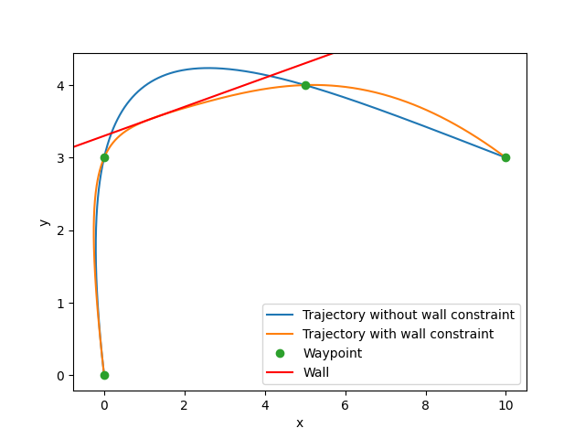
Output:
It can be seen that while the trajectory without the constraint goes through the wall, the trajectory with the constraint avoids the wall correctly.