 Similarly,
 Similarly,
 Similarly,
 Similarly,
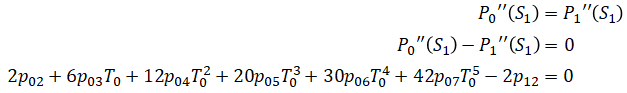
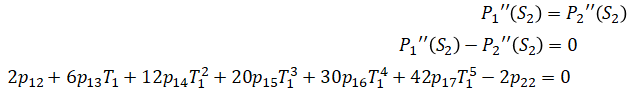
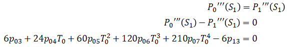
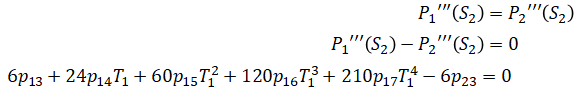
This page describes a method to generate polynomial trajectories by solving a Quadratic Programming (QP) problem. Concepts are explained through two examples. The frist example shows how to generate a minimum acceleration trajectory that passes through two points. The second example shows how to generate a minimum snap trajectory that passes through several waypoints. Python code is provided.
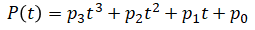
The first example is to find a trajectory with minimum acceleration that moves from x0=1 to xf=2 in T=10 seconds. The minimum degree of a polynomial to ensure smoothness for a minimum acceleration (2nd derivative) trajectory is 3 (i.e. cubic polynomial):
The goal is to find the four coefficients p0 to p3. To do so, we rephrase the problem as a QP problem of the form:
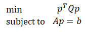
where p is the vector of the polynomial coefficients:

Once we rephrase it, the problem can be solved efficiently with readily available QP libraries.
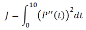
Since we want to minimize the acceleration, the cost function can be written as:
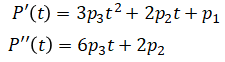
The derivatives of P(t) can be calculated as,
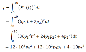
Substituting this into the cost function yields:
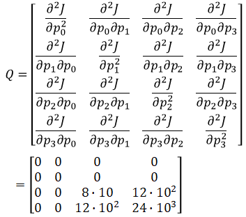
The Q matrix is found by taking the hessian matrix of J:
Next are the constraints:

which is equivalent to,
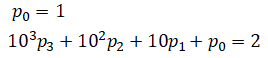
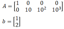
This can be rewritten in matrix form as:
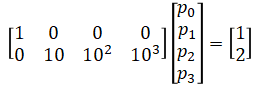
So the A matrix and b vector are given by:
Below is a Python script to solve the QP for the above example:
import numpy as np
from cvxopt import matrix, solvers

x0 = 1.0
xf = 2.0
T = 10.0

Q = np.array([
    [0, 0, 0, 0],
    [0, 0, 0, 0],
    [0, 0, 8*T, 12*(T**2)],
    [0, 0, 12*(T**2), 24*(T**3)],
])

f = np.zeros(4)

A = np.array([
    [1, 0, 0, 0],
    [1, T, T**2, T**3]
])
b = np.array([x0, xf])

sol = solvers.qp(matrix(Q), matrix(f), None, None, matrix(A), matrix(b))
print(sol['x'])
The resulting polynomial is:
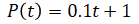
which is a line (zero acceleration) that passes through P(0)=1 and P(10)=2.
The next example is to generate a minimum snap (4th derivative) trajectory that passes through 4 waypoints at the following times:
| i | t | x |
|---|---|---|
| 0 | 0 | 0 |
| 1 | 10 | 5 |
| 2 | 30 | 5 |
| 3 | 40 | 3 |
Since there are 4 waypoints, it is going to be a piecewise polynomial function of 3 parts. Each polynomial joins two consecutive waypoints. We will use a septic polynomial (7th degree polynomial) for each segment because that is the minimum degree required to satisfy the minimum snap requirement. Polynomial Pi(t) joins waypoints i and i+1:

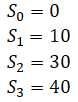
where Si are the times at the beginning of each trajectory:
There are 3*8=24 unknown coefficients. Again the problem is set up as a QP problem:
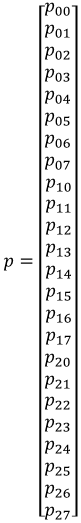
Where p is a vector of all 24 coefficients:
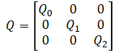
The Q matrix will be a 24x24 matrix. It is a block diagonal matrix made of three parts (one for each polynomial).
Each submatrix can be calculated this time using symbolic math:
import sympy

t, T = sympy.symbols('t T')
p0, p1, p2, p3, p4, p5, p6, p7 = sympy.symbols('p0 p1 p2 p3 p4 p5 p6 p7')

P = p7*t**7 + p6*t**6 + p5*t**5 + p4*t**4 + p3*t**3 + p2*t**2 + p1*t + p0
P1 = sympy.diff(P, t) # Speed
P2 = sympy.diff(P1, t) # Acceleration
P3 = sympy.diff(P2, t) # Jerk
P4 = sympy.diff(P3, t) # Snap
J = sympy.integrate(P4**2, (t, 0, T))
Q = sympy.hessian(J, (p0, p1, p2, p3, p4, p5, p6, p7))

sympy.pprint(Q)
This results in:
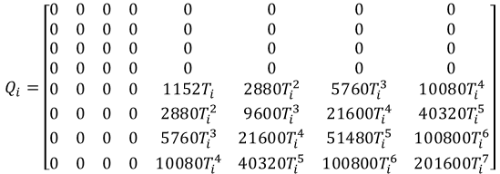
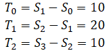
where Ti is the time interval between waypoints i and i+1:
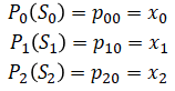
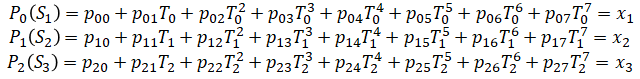
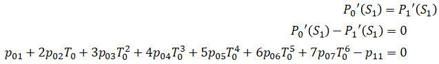
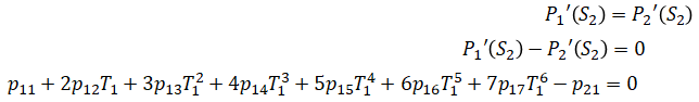
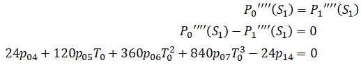
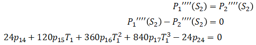
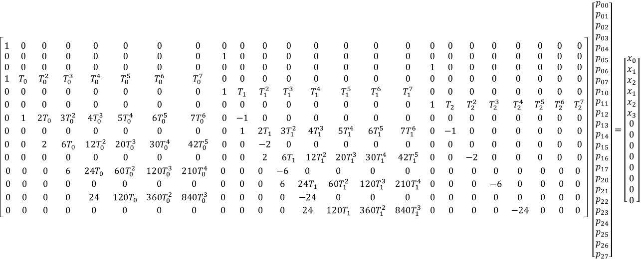
Next are the constraints (Ap=b). We will apply 14 constraints in total. A is 14x24 matrix where each row is a constraint.
Similarly,
Similarly,
Similarly,
Similarly,
Putting all of this together in matrix form Ap = b:
Solving the QP:
import numpy as np
from cvxopt import matrix, solvers
import matplotlib.pyplot as plt

def get_Q(T):
    return np.array([
        [0, 0, 0, 0, 0, 0, 0, 0],
        [0, 0, 0, 0, 0, 0, 0, 0],
        [0, 0, 0, 0, 0, 0, 0, 0],
        [0, 0, 0, 0, 0, 0, 0, 0],
        [0, 0, 0, 0, 1152*T, 2880*T**2, 5760*T**3, 10080*T**4],
        [0, 0, 0, 0, 2880*T**2, 9600*T**3, 21600*T**4, 40320*T**5],
        [0, 0, 0, 0, 5760*T**3, 21600*T**4, 51840*T**5, 100800*T**6],
        [0, 0, 0, 0, 10080*T**4, 40320*T**5, 100800*T**6, 201600*T**7]
    ])

def get_coefficients(T, wp):
    N = 8 # Septic polynomial has 8 coefficients
    M = len(T) # Number of polynomial segments
    L = 14 # Number of constraints

    # Q Matrix
    Z = np.zeros((N, N))
    Q0 = get_Q(T[0])
    Q1 = get_Q(T[1])
    Q2 = get_Q(T[2])
    Q = np.block([
        [Q0, Z, Z],
        [Z, Q1, Z],
        [Z, Z, Q2]
    ])

    f = np.zeros(N*M)

    # Constraints (Ap=b)
    A = np.zeros((L, N*M))
    # Start position of polynomials
    A[0,:8] = [1, 0, 0, 0, 0, 0, 0, 0]
    A[1,8:16] = [1, 0, 0, 0, 0, 0, 0, 0]
    A[2,16:] = [1, 0, 0, 0, 0, 0, 0, 0]
    # End position of polynomials
    A[3,:8] = [1, T[0], T[0]**2, T[0]**3, T[0]**4, T[0]**5, T[0]**6, T[0]**7]
    A[4,8:16] = [1, T[1], T[1]**2, T[1]**3, T[1]**4, T[1]**5, T[1]**6, T[1]**7]
    A[5,16:] = [1, T[2], T[2]**2, T[2]**3, T[2]**4, T[2]**5, T[2]**6, T[2]**7]
    # Continuous velocity
    A[6,:16] = [0, 1, 2*T[0], 3*T[0]**2, 4*T[0]**3, 5*T[0]**4, 6*T[0]**5, 7*T[0]**6, 0, -1, 0, 0, 0, 0, 0, 0]
    A[7,8:] = [0, 1, 2*T[1], 3*T[1]**2, 4*T[1]**3, 5*T[1]**4, 6*T[1]**5, 7*T[1]**6, 0, -1, 0, 0, 0, 0, 0, 0]
    # Continuous acceleration
    A[8,:16] = [0, 0, 2, 6*T[0], 12*T[0]**2, 20*T[0]**3, 30*T[0]**4, 42*T[0]**5, 0, 0, -2, 0, 0, 0, 0, 0]
    A[9,8:] = [0, 0, 2, 6*T[1], 12*T[1]**2, 20*T[1]**3, 30*T[1]**4, 42*T[1]**5, 0, 0, -2, 0, 0, 0, 0, 0]
    # Continuous jerk
    A[10,:16] = [0, 0, 0, 6, 24*T[0], 60*T[0]**2, 120*T[0]**3, 210*T[0]**4, 0, 0, 0, -6, 0, 0, 0, 0]
    A[11,8:] = [0, 0, 0, 6, 24*T[1], 60*T[1]**2, 120*T[1]**3, 210*T[1]**4, 0, 0, 0, -6, 0, 0, 0, 0]
    # Continuous snap
    A[12,:16] = [0, 0, 0, 0, 24, 120*T[0], 360*T[0]**2, 840*T[0]**3, 0, 0, 0, 0, -24, 0, 0, 0]
    A[13,8:] = [0, 0, 0, 0, 24, 120*T[1], 360*T[1]**2, 840*T[1]**3, 0, 0, 0, 0, -24, 0, 0, 0]

    b = np.zeros(L)
    b[:6] = [wp[0], wp[1], wp[2], wp[1], wp[2], wp[3]]

    sol = solvers.qp(matrix(Q), matrix(f), None, None, matrix(A), matrix(b))
    return list(sol['x'])

# Waypoints
wp_t = np.array([0., 10., 30., 40.])
wp_x = np.array([0., 5., 5., 3.])
T = np.ediff1d(wp_t)

p = get_coefficients(T, wp_x)

N = 500
t = np.linspace(wp_t[0], wp_t[-1], N)
pos = [None] * N
vel = [None] * N
acc = [None] * N
jrk = [None] * N
snp = [None] * N
for i in range(N):
    j = np.nonzero(t[i] <= wp_t)[0][0] - 1
    j = np.max([j, 0])
    ti = t[i] - wp_t[j]
    x_coeff = np.flip(p[8*j:8*j+8])
    v_coeff = np.polyder(x_coeff)
    a_coeff = np.polyder(v_coeff)
    j_coeff = np.polyder(a_coeff)
    s_coeff = np.polyder(j_coeff)
    pos[i] = np.polyval(x_coeff, ti)
    vel[i] = np.polyval(v_coeff, ti)
    acc[i] = np.polyval(a_coeff, ti)
    jrk[i] = np.polyval(j_coeff, ti)
    snp[i] = np.polyval(s_coeff, ti)

plt.subplot(5, 1, 1)
plt.plot(t, pos, label='Position')
plt.plot(wp_t, wp_x, '.', label='Waypoint')
plt.legend()
plt.subplot(5, 1, 2)
plt.plot(t, vel, label='velocity')
plt.legend()
plt.subplot(5, 1, 3)
plt.plot(t, acc, label='acceleration')
plt.legend()
plt.subplot(5, 1, 4)
plt.plot(t, jrk, label='jerk')
plt.legend()
plt.subplot(5, 1, 5)
plt.plot(t, snp, label='snap')
plt.legend()
plt.xlabel('Time')
plt.show()
Output:
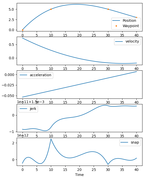
It can be seen that the trajectory passes through all the waypoints and it is continuous up to the snap.