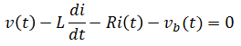
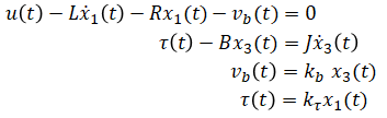
(eq. 1)
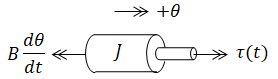 From this free body diagram:
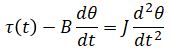
(eq. 2)
(eq. 3)
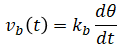
(eq. 4)
Transfer function and state space model are developed for a permanent magnet DC motor. This system is a combination of an LR circuit and mass with rotational friction.
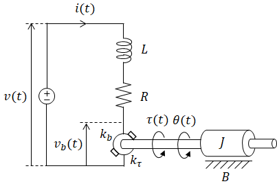
| (input) | v(t) | = | applied voltage (armature voltage) (V) | |
| i(t) | = | armature current (A) | unknowns | |
| vb(t) | = | back emf (V) | ||
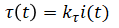
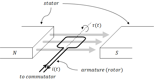
| τ(t) | = | generated torque (Nm) | ||
| (output) | θ(t) | = | rotor position (rad) | |
| L | = | armature inductance | ||
| R | = | armature resistance | ||
| J | = | load and armature inertia | ||
| B | = | motor friction coefficient (e.g. brushes) | ||
| kτ | = | motor torque constant (Nm/A) | ||
| kb | = | motor back emf constant (V*sec/rad) |
Permanent magnet produces constant flux so flux is included in the motor constants.
4 unknowns so 4 equations are needed.
From this free body diagram:
Laplace transform (eq. 1), (eq. 2), (eq. 3), (eq. 4):
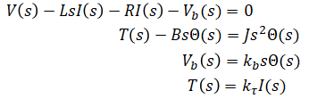
Solve for the 4 unknowns:
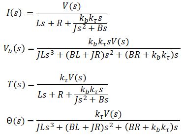
Solve for output/input:
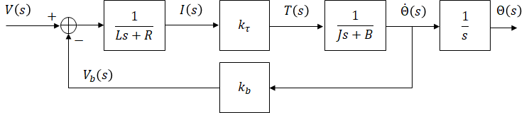
Block diagram is drawn from input to output. Voltage creates current flow, current produces torque, and torque rotates the motor which dictates its position. Some techniques used below to create and manipulate block diagrams are covered here.
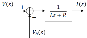
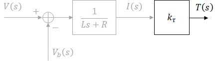
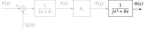
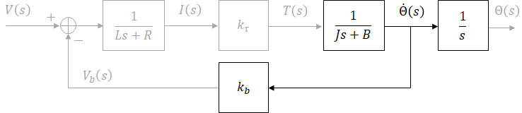
This is not the only block diagram that can be constructed for this system but the blocks in this diagram closely represent physical parts of the system.
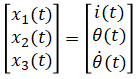
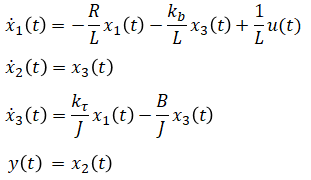
When an inductor is present in a system, current through the inductor is commonly chosen as a state variable. When a mass is present, its position and velocity are commonly chosen as state variables. These three variables along with the input are enough to determine this system's behavior (future values of the output, which is the position of the motor in this system). For these reasons, current, rotor position, and rotor angular velocity are chosen as the state variables.
State vector:
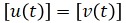
Input vector:
Output vector:
Rewrite (eq. 1), (eq. 2), (eq. 3), (eq. 4) in these new notations:
Rearrange equations to express ẋ(t) and y(t) in terms of x(t) and u(t):
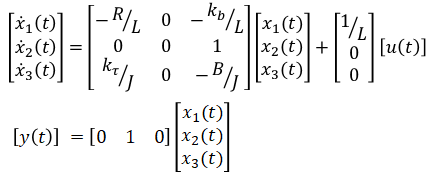
Rewrite in matrix format:
The 3rd order system can be approximated as a 2nd order system as follows[1][2]
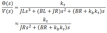
[1] Phillips, Parr (2011) Feedback Control Systems 5th Edition: inductance is
small enough to be ignored for servomotors
[2] Spong, Hutchinson, Vidyasagar (2006) Robot Modeling and Control: it is
reasonable to assume L/R (electrical time constant) << J/B
(mechanical time constant) for many electro-mechanical systems so let L/R be 0.