This page describes a method to generate quintic (5th degree) polynomial
trajectory. Two examples are provided: a 1D trajectory and a 3D helix
trajectory. Velocity and acceleration are also calculated.
Code is provided in Python.
Our goal is to generate a smooth path that joins two points in space.
We will use a quintic polynomial to describe such path.
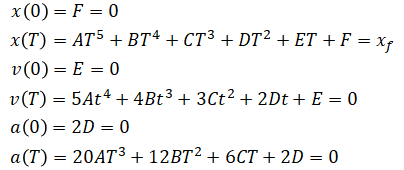
A quintic polynomial has the form:
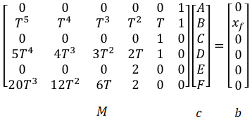
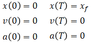
Since there are six unknowns, we need six equations. These are constraints
that we must enforce. We will pick the following 6 constraints:
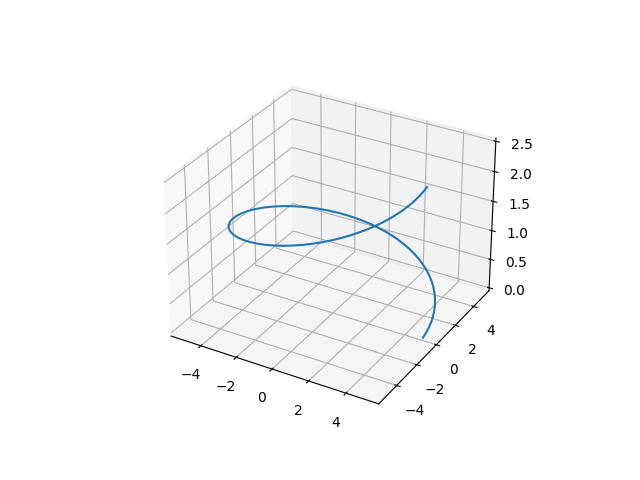
A particle moves in a helix of radius 5 around Z-axis from (x,y,z) = (5,0,0) to
(5,0,2.5) in T=12 seconds (makes one round circle).
The angle (theta) is going to be a quintic polynomial trajectory.
The height (z) is also going to be a quintic polynomial trajectory.
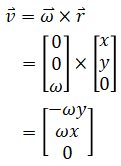
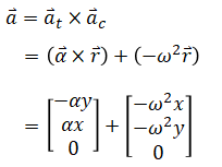
Acceleration is made of tangent and centripetal parts. It can be calculated as:
import numpy as np
import matplotlib.pyplot as plt
# For a polynomial of
# x(t) = At^5 + Bt^4 + Ct^3 + Dt^2 + Et + F
# returns coefficients:
# [A, B, C, D, E, F]
# Constraints:
# - Initial position is 0: x(0) = 0
# - Final position is xf: x(T) = xf
# - Initial and final velocities are 0
# - Initial and final accelerations are 0
def get_quintic_poly_coeff(T, xf):
M = np.array([
[ 0, 0, 0, 0, 0, 1],
[ 0, 0, 0, 0, 1, 0],
[ 0, 0, 0, 2, 0, 0],
[ T**5, T**4, T**3, T**2, T, 1],
[ 5*T**4, 4*T**3, 3*T**2, 2*T, 1, 0],
[20*T**3, 12*T**2, 6*T, 2, 0, 0]
])
b = np.array([0, 0, 0, xf, 0, 0])
coeff = np.linalg.solve(M, b)
return coeff
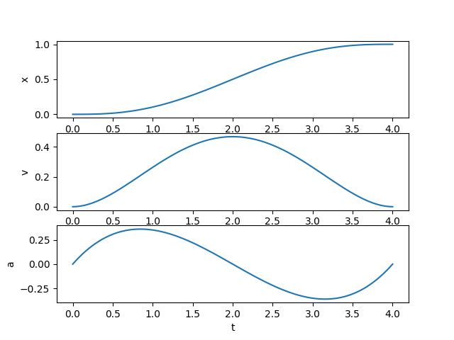
def plot_line_trajectory():
# Move from x=0 to x=1 in T=4 seconds
T = 4
xf = 1
# Calculate coefficients
x_coeff = get_quintic_poly_coeff(T, xf)
v_coeff = np.polyder(x_coeff)
a_coeff = np.polyder(v_coeff)
N = 100
t = np.linspace(0, T, N)
x = [None] * N
v = [None] * N
a = [None] * N
# Generate trajectory
for i in range(N):
x[i] = np.polyval(x_coeff, t[i])
v[i] = np.polyval(v_coeff, t[i])
a[i] = np.polyval(a_coeff, t[i])
# Plot
plt.subplot(3, 1, 1)
plt.plot(t, x)
plt.ylabel('x')
plt.subplot(3, 1, 2)
plt.plot(t, v)
plt.ylabel('v')
plt.subplot(3, 1, 3)
plt.plot(t, a)
plt.ylabel('a')
plt.xlabel('t')
plt.show()
def plot_helix_trajectory():
# Moves in a helix of radius 5 around Z-axis from (x,y,z) = (5,0,0) to
# (5,0,2.5) in T=12 seconds (makes one round circle)
R = 5
T = 12
thetaf = 2*np.pi
zf = 2.5
# Calculate coefficients
theta_coeff = get_quintic_poly_coeff(T, thetaf)
omega_coeff = np.polyder(theta_coeff)
alpha_coeff = np.polyder(omega_coeff)
z_coeff = get_quintic_poly_coeff(T, zf)
vz_coeff = np.polyder(z_coeff)
az_coeff = np.polyder(vz_coeff)
N = 100
t = np.linspace(0, T, N)
x, y, z = [None] * N, [None] * N, [None] * N
vx, vy, vz = [None] * N, [None] * N, [None] * N
ax, ay, az = [None] * N, [None] * N, [None] * N
# Generate trajectory
for i in range(N):
theta = np.polyval(theta_coeff, t[i])
omega = np.polyval(omega_coeff, t[i])
alpha = np.polyval(alpha_coeff, t[i])
z[i] = np.polyval(z_coeff, t[i])
vz[i] = np.polyval(vz_coeff, t[i])
az[i] = np.polyval(az_coeff, t[i])
x[i] = np.cos(theta) * R
y[i] = np.sin(theta) * R
vx[i] = -y[i]*omega
vy[i] = x[i]*omega
ax[i] = -x[i]*omega**2 - y[i]*alpha
ay[i] = -y[i]*omega**2 + x[i]*alpha
# Plot
ax = plt.axes(projection='3d')
ax.plot(x, y, z)
plt.show()
plot_line_trajectory()
plot_helix_trajectory()


 So this constraint can be rewritten as


 So this constraint can be rewritten as