This page lists Python code snippets for controls engineering.
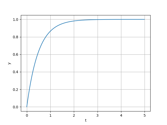
import control
import numpy as np
import matplotlib.pyplot as plt

tau = 0.5
K = 1
num = [K]
den = [tau, 1]
sys = control.tf(num, den)

dt = 0.01
t = np.arange(0, 5, dt)
t, y = control.step_response(sys, t)

plt.plot(t, y)
plt.xlabel('t')
plt.ylabel('y')
plt.grid()
plt.show()
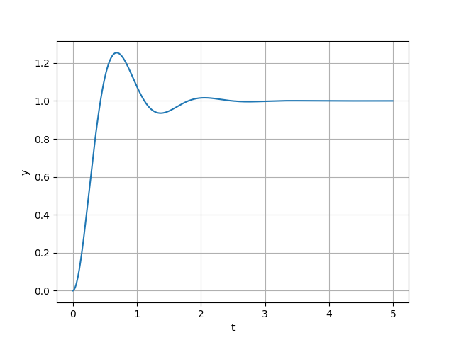
import control
import numpy as np
import matplotlib.pyplot as plt

zeta = 0.4
omega_n = 5
num = [omega_n**2]
den = [1, 2*zeta*omega_n, omega_n**2]
sys = control.tf(num, den)

dt = 0.01
t = np.arange(0, 5, dt)
t, y = control.step_response(sys, t)

plt.plot(t, y)
plt.xlabel('t')
plt.ylabel('y')
plt.grid()
plt.show()
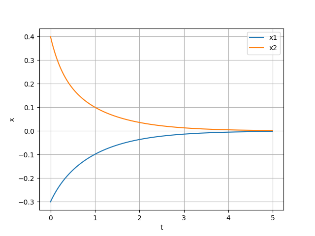
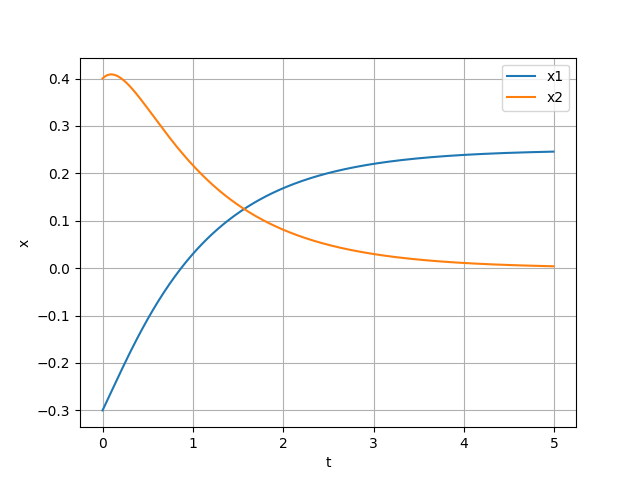
import control
import numpy as np
import matplotlib.pyplot as plt

A = [[0, 1], [-4, -5]]
B = [[0], [1]]
C = np.eye(2)
D = np.zeros([2, 1])
sys = control.ss(A, B, C, D)

dt = 0.01
t = np.arange(0, 5, dt)
X0 = [-0.3, 0.4]
t, x = control.initial_response(sys, t, X0)

plt.plot(t, x[0], label='x1')
plt.plot(t, x[1], label='x2')
plt.xlabel('t')
plt.ylabel('x')
plt.grid()
plt.legend()
plt.show()
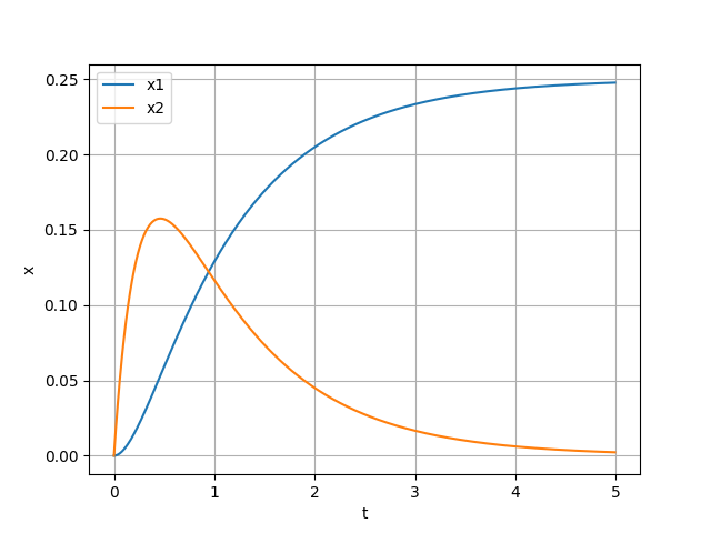
import control
import numpy as np
import matplotlib.pyplot as plt

A = [[0, 1], [-4, -5]]
B = [[0], [1]]
C = np.eye(2)
D = np.zeros([2, 1])
sys = control.ss(A, B, C, D)

dt = 0.01
t = np.arange(0, 5, dt)
t, x = control.step_response(sys, t)

plt.plot(t, x[0,0,:], label='x1')
plt.plot(t, x[1,0,:], label='x2')
plt.xlabel('t')
plt.ylabel('x')
plt.grid()
plt.legend()
plt.show()
import control
import numpy as np
import matplotlib.pyplot as plt

A = [[0, 1], [-4, -5]]
B = [[0], [1]]
C = np.eye(2)
D = np.zeros([2, 1])
sys = control.ss(A, B, C, D)

dt = 0.01
t = np.arange(0, 5, dt)
X0 = [-0.3, 0.4]
t, x = control.step_response(sys, t, X0)

plt.plot(t, x[0,0,:], label='x1')
plt.plot(t, x[1,0,:], label='x2')
plt.xlabel('t')
plt.ylabel('x')
plt.grid()
plt.legend()
plt.show()
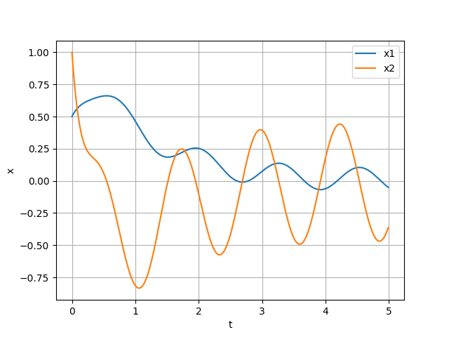
import control
import numpy as np
import matplotlib.pyplot as plt

A = [[0, 1], [-4, -5]]
B = [[0], [1]]
C = np.eye(2)
D = np.zeros([2, 1])
sys = control.ss(A, B, C, D)

dt = 0.01
t = np.arange(0, 5, dt)
u = 3 * np.sin(5*t)
X0 = [0.5, 1]
t, x = control.forced_response(sys, t, u, X0)

plt.plot(t, x[0], label='x1')
plt.plot(t, x[1], label='x2')
plt.xlabel('t')
plt.ylabel('x')
plt.grid()
plt.legend()
plt.show()
Stable if all poles have negative real part.
import control
import numpy as np

num = [1]
den = [1, 1]
sys = control.tf(num, den)
print(sys.pole())
print(np.roots(den)) # Alternate method
Output:
[-1.+0.j]
[-1.]
Example is stable.
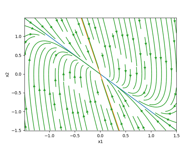
Stable if all eigenvalues of the system matrix have negative real part.
import numpy as np

A = np.array([
    [0, 1],
    [-4, -5]
])
print(np.linalg.eigvals(A))
Output:
[-1. -4.]
Example is stable.
import numpy as np
import matplotlib.pyplot as plt

w = 1.5
Y, X = np.mgrid[-w:w:100j, -w:w:100j]

A = np.array([
    [0, 1],
    [-4, -5]
])
s, v = np.linalg.eig(A)

U = A[0,0]*X + A[0,1]*Y
V = A[1,0]*X + A[1,1]*Y

if s.imag[0] == 0 and s.imag[1] == 0:
    t = np.arange(-1.5, 1.5, 0.01)
    plt.plot(t, (v[1,0]/v[0,0])*t)
    plt.plot(t, (v[1,1]/v[0,1])*t)
plt.streamplot(X, Y, U, V)
plt.xlabel('x1')
plt.ylabel('x2')
plt.show()
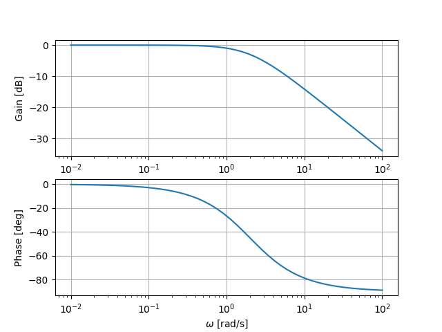
import control
import numpy as np
import matplotlib.pyplot as plt

num = [1]
den = [0.5, 1]
sys = control.tf(num, den)

dt = 0.01
t = np.arange(0, 5, dt)
omega = np.logspace(-2, 2)
gain, phase, omega = control.bode_plot(sys, omega, plot=False)
plt.subplot(2, 1, 1)
plt.semilogx(omega, control.mag2db(gain))
plt.ylabel('Gain [dB]')
plt.grid()
plt.subplot(2, 1, 2)
plt.semilogx(omega, np.degrees(phase))
plt.xlabel('$\omega$ [rad/s]')
plt.ylabel('Phase [deg]')
plt.grid()
plt.show()