This page describes a method to estimate continuous-time transfer function of an unknown system from its input and output data. The degree of the numerator and denominator of the transfer function is assumed to be known. An example is provided with code in Python.
Transfer function H[ω] (or frequency response function, FRF) of a system with input x[n] and output y[n] data can be calculated by:
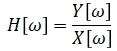
where X = fft(x) and Y = fft(y).
We can use a minimization solver to estimate a transfer function H(s) which has a frequency response that closely resembles H[ω]. We can evaluate H(s) at a particular frequency by substituting s for jω.
We apply a chirp signal to an unknown system and use only the input & output measurements to estimate the transfer function.
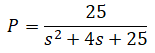
First, suppose that the unknown system is actually a second order system given by:
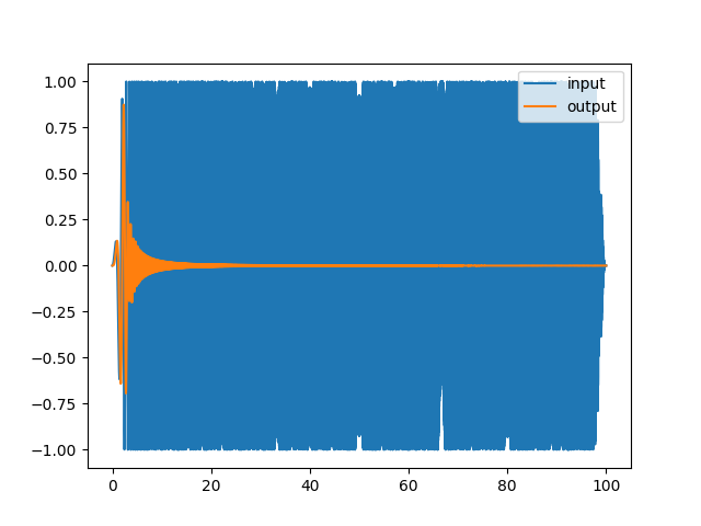
Next we apply a chirp signal (frequency ramp) to this system at 100Hz sampling rate for 100 seconds. The chirp function frequency is varied from 0 to 50Hz.
Input and output signal vs time:
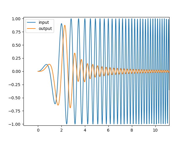
Zoomed in:
Chirp function is chosen because it provides more power per frequency bin than a direct impulse response. Frequency is varied up to 50Hz because that is half the sampling rate.
The chirp signal is windowed to minimize distortion in the FFT results. Tukey window is chosen because it tapers only the outer edges. We do not want to taper the boundaries too much because the chirp signal sweeps the frequency with time and any tapered region would have reduced signal levels.
Below is bode diagram of true frequency response generated from the second order transfer function P and estimated frequency response function H generated by FFT of input and output data. H is used to estimate the continuous transfer function.
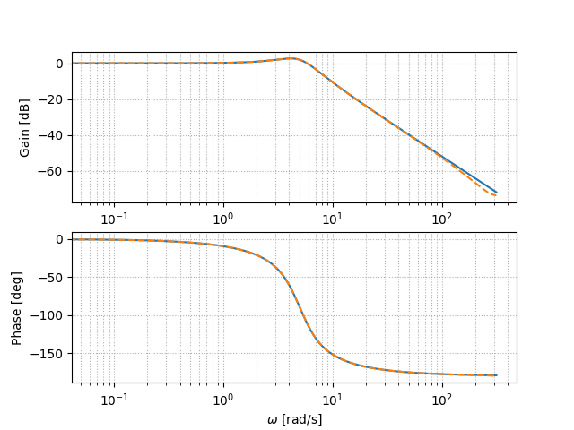
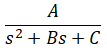
Finally minimization solver is set up to find the constants A, B, and C in the transfer function of the following form:
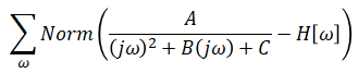
Objective function is to minimize the difference between estimated transfer function and H:
import control
import scipy
import numpy as np
import matplotlib.pyplot as plt

# True model
sys = control.tf([25], [1, 4, 25])
print('True:')
print(sys)

# Time
T = 100.0                   # Duration [sec]
fs = 100                    # Sampling rate [Hz]
dt = 1/fs                   # Time step [sec]
N = int(T * fs)             # Number of samples
t = np.arange(N) * dt       # List of times [sec]

# Generate chirp function from 0 to 50Hz (input function)
chirp = scipy.signal.chirp(t, f0=0, t1=t[-1], f1=50)
tukey = scipy.signal.windows.tukey(N, 0.05)
u = chirp * tukey

# Generate response of chirp input
t, y = control.forced_response(sys, t, u)

# Plot system input and output
plt.plot(t, u, label='input')
plt.plot(t, y, label='output')
plt.legend()
plt.show()

# Frequency
f = np.fft.fftfreq(N, d=dt) # List of frequencies [Hz]
omega = 2 * np.pi * f       # List of frequencies [rad/sec]
half = N // 2

# Estimate FRF (frequency response function) using input and output
U = np.fft.fft(u) # Input spectrum
Y = np.fft.fft(y) # Output spectrum
H = Y / U

# Use only the first half of FFT
H = H[:half]
omega = omega[:half]

# Generate true frequency response
mag, phase, _ = control.bode(sys, omega, plot=False)

# Get frequency response from estimated FRF
mag2 = abs(H)
phase2 = np.angle(H)

# Compare true vs estimated frequency response with bode plot
fig, ax = plt.subplots(2, 1)
ax[0].semilogx(omega, control.mag2db(mag))
ax[0].semilogx(omega, control.mag2db(mag2), '--')
ax[0].set_ylabel('Gain [dB]')
ax[0].grid(which='both', ls=':')
ax[1].semilogx(omega, np.rad2deg(phase))
ax[1].semilogx(omega, np.rad2deg(phase2), '--')
ax[1].set_ylabel('Phase [deg]')
ax[1].set_xlabel('$\\omega$ [rad/s]')
ax[1].grid(which='both', ls=':')
plt.show()

# Objective function to be minimized
def fun(x):
    # x[0] / (s^2 + x[1]*s + x[2])
    s = 1j * omega
    frf = x[0] / np.polyval([1, x[1], x[2]], s)
    return np.linalg.norm(frf - H).sum()

# Estimated model in the form K / (s^2 + a*s + b) using H and omega
x0 = [1, 1, 1]
result = scipy.optimize.minimize(fun, x0)
num = [result.x[0]]
den = [1, result.x[1], result.x[2]]
sys_est = control.tf(num, den)
print('Estimated:')
print(sys_est)
Output:
True:

      25
--------------
s^2 + 4 s + 25

Estimated:

    24.99
--------------
s^2 + 4 s + 25
It shows that the estimated transfer function closely resembles the true transfer function.
The method of calculating H by Y/X does not work well when there is noise in the data. A common solution is to use H1 or H2 frequency response estimators. Examples are shown below:
# H_1 estimator

_, Pxy = scipy.signal.csd(u, y, fs=1/dt, nperseg=N, window='boxcar')
_, Pxx = scipy.signal.welch(u, fs=1/dt, nperseg=N, window='boxcar')
H = Pxy/Pxx

# H_2 estimator

_, Pyx = scipy.signal.csd(y, u, fs=1/dt, nperseg=N, window='boxcar')
_, Pyy = scipy.signal.welch(y, fs=1/dt, nperseg=N, window='boxcar')
H = Pyy / Pyx