This page describes a method to estimate step response of an unknown system with only its input and output data. This is useful when it is not possible to directly apply and observe the step response of a system but would still like to know how it looks. An example of this is when tuning angular rate PID controller of a drone. Example code in Python is also provided.
FFT cross-correlation is used to compute the impulse response of the system. This is called FIR (finite impulse response) system identification. The impulse response is then integrated to give the step response.
From signal processing, we know that the output y[n] of any LTI filter can be computed by convolving the input signal x[n] with its impulse response h[n]:

Using the convolution theorem we know that

where upppercase denotes frequency-domain signal and "·" is element-wise multiplication. We can calculate the frequency response H by Y/X (that is fft(y)/fft(x)) but this does not work well when there is noise in the measured output (which is always the case).
The cross-correlation of input signal with the output signal is

Using the cross-correlation theorem we can write this as

where the bar over the variable denotes complex conjugate. Substituting H·X to Y and rearranging the terms, we find that
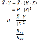
So the frequency response H is the input-output cross-power spectrum divided by the input power spectrum."·" is element-wise multiplication and "/" is element-wise division.
Inverse FFT of the frequency response yields the impulse response h[n]. Only the real part is used because any imaginary part is quantization noise.
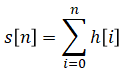
Finally, the step response s[n] can be calculated by integrating the impulse response h[n]:
We apply a chirp signal to an unknown system and use only the input & output measurements to estimate the step response.
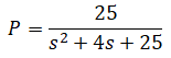
First, suppose that the unknown system is actually a second order system given by:
Next we apply a chirp signal (frequency ramp) to this system at 100Hz sampling rate for 100 seconds. The chirp function frequency is varied from 0 to 50Hz.
Input and output signal vs time:
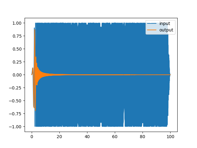
Zoomed in:
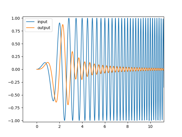
Chirp function is chosen because it provides more power per frequency bin than a direct impulse response. Frequency is varied up to 50Hz because that is half the sampling rate.
The chirp signal is windowed to minimize distortion in the FFT results. Tukey window is chosen because it tapers only the outer edges. We do not want to taper the boundaries too much because the chirp signal sweeps the frequency with time and any tapered region would have reduced signal levels.
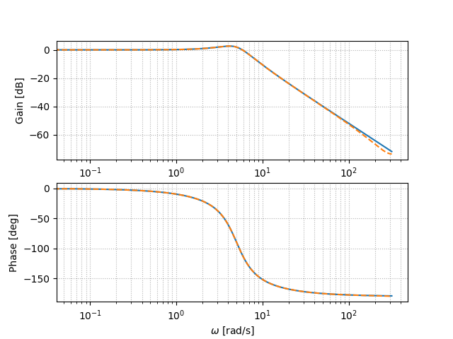
Frequency response H is calculated using the input and output data. Below is a bode diagram of real (solid) and estimated (dashed) frequency response. They closely resemble.
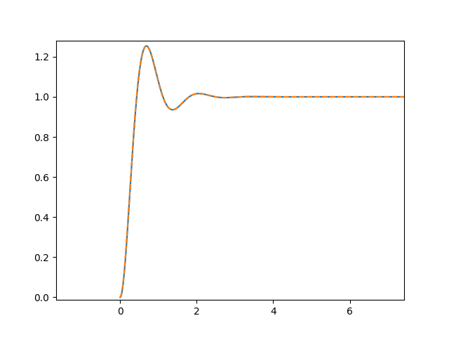
Frequency response is converted to impulse response and then to step response. Below shows that the real and estimated step response closely resemble.
import numpy as np
import scipy
import control
import matplotlib.pyplot as plt

# True model (second order model)
num = [25]
den = [1, 4, 25]
sys = control.tf(num, den)

# Time
T = 100.0                   # Duration [sec]
fs = 100                    # Sampling rate [Hz]
dt = 1/fs                   # Time step [sec]
N = int(T * fs)             # Number of samples
t = np.arange(N) * dt       # List of times [sec]

# Frequency
f = np.fft.fftfreq(N, d=dt) # List of frequencies [Hz]
omega = 2 * np.pi * f       # List of frequencies [rad/sec]
half = N // 2

# Generate true step response
t, step = control.step_response(sys, t)

# Generate true frequency response
mag, phase, _ = control.bode(sys, omega[:half], plot=False)

# Generate chirp function from 0 to 50Hz (input function)
chirp = scipy.signal.chirp(t, f0=0, t1=t[-1], f1=50)
tukey = scipy.signal.windows.tukey(N, 0.05)
u = chirp * tukey

# Generate response of chirp input
t, y = control.forced_response(sys, t, u)

# Plot chirp input and output
plt.plot(t, u, label='input')
plt.plot(t, y, label='output')
plt.legend()
plt.show()

# Estimate model using chirp input and output
U = np.fft.fft(u) # Input spectrum
Y = np.fft.fft(y) # Output spectrum
Rxx = U.conjugate() * U     # Energy spectrum of u
Rxy = U.conjugate() * Y     # Cross-energy spectrum
Hxy = Rxy / Rxx             # Frequency response

# Get step response from estimated model
hxy = np.fft.ifft(Hxy).real # Impulse response
step2 = np.cumsum(hxy)      # Step response

# Get frequency response from estimated model
mag2 = abs(Hxy[:half])
phase2 = np.angle(Hxy[:half])

# Compare true vs estimated frequency response with bode plot
w = omega[:half]
fig, ax = plt.subplots(2, 1)
ax[0].semilogx(w, control.mag2db(mag))
ax[0].semilogx(w, control.mag2db(mag2), '--')
ax[0].set_ylabel('Gain [dB]')
ax[0].grid(which='both', ls=':')
ax[1].semilogx(w, np.rad2deg(phase))
ax[1].semilogx(w, np.rad2deg(phase2), '--')
ax[1].set_ylabel('Phase [deg]')
ax[1].set_xlabel('$\\omega$ [rad/s]')
ax[1].grid(which='both', ls=':')
plt.show()

# Compare true vs estimated step response
plt.plot(t, step)
plt.plot(t, step2, '--')
plt.show()