This page describes a method to estimate position and velocity in 1D given position and velocity measurements from devices like GNSS and acceleration measurements from accelerometer. Kalman filter is used with constant velocity model. A working Python code is also provided.
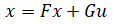
Given system and measurement equations,
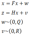
Discrete-time Kalman filter steps are,
| 1. | Prediction: state | |
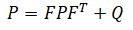
| 2. | Prediction: covariance | |
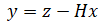
| 3. | Innovation | |
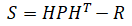
| 4. | Innovation: covariance | |
| 5. | Kalman gain | |
| 6. | Update: state | |
| 7. | Update: state | |
Accelerometer data are assumed to be in m/s2. Accelerometer data are not treated as observations. Instead, they are used as inputs in the prediction step.
State vector is:

The first parameter is position (m) and the second parameter is velocity (m/sec).
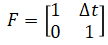
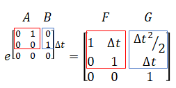
State transition matrix F is needed to predict the state and covariance. F is a 2x2 matrix given by:
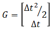
Control input model matrix G is needed to calculate the process noise Q. G is a 2x1 matrix given by:
F and G are derived as follows:
Let

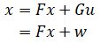
then the equation of motion in state-space form is
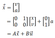
where A is the system matrix and B is continuous input matrix. It is a constant velocity model with acceleration as input. A and B can be discretized using the following property:
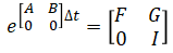
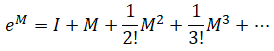
Matrix exponential can be solved using the following property:
Using these properties, it can be found that
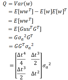
Discrete constant white noise model (piecewise white noise model) is used. Acceleration is assumed to be constant for the duration of each time period but differs for each time period. Each of these is uncorrelated between time periods. At each time step, there is a discontinuous jump in acceleration.
From the previous section, we have
where
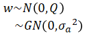
σa is the IMU accelerometer noise (1 standard deviation) in units of m/s2. The process noise matrix is:
Reference: Bar-Shalom. “Estimation with Applications To Tracking and Navigation”. John Wiley & Sons, 2001. Page 274.
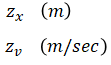
There are two types of observations: position and velocity (both scalar).
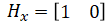
The measurement equation for position observation is,
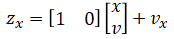
so the observation model is
The measurement equation for velocity observation is,
so the observation model is
Observation noise is given by,

σx is 1-standard deviation position error (positional accuracy estimate) in m obtained from GNSS receiver (often called eph).
σv is 1-standard deviation speed error (speed accuracy estimate) in m/sec obtained from GNSS receiver (often called sAcc).
filter.py
import numpy as np


class KF:
    def __init__(self, x0=0, v0=0, x0_acc=0.5, v0_acc=0.5, a_acc=0.35):
        '''
        x0 -- initial position [m]
        v0 -- initial velocity [m/sec]
        x0_acc -- initial position accuracy (1-standard deviation) [m]
        v0_acc -- initial velocity accuracy (1-standard deviation) [m/sec]
        a_acc -- accelerometer noise (1-standard deviation). [m/sec^2]
        '''
        self.x = np.array([[x0], [v0]]) # State
        self.P = np.diag([x0_acc ** 2, v0_acc ** 2])
        self.W = np.array([[a_acc ** 2]])

    def predict(self, a, dt):
        '''
        a -- accelerometer measurement [m/sec^2]
        dt -- time step [sec]
        '''
        F = np.array([
            [1, dt],
            [0,  1]
        ])
        G = np.array([
            [dt*dt/2],
            [dt]
        ])
        u = np.array([[a]])
        self.x = F @ self.x + G @ u
        self.P = F @ self.P @ F.T + G @ self.W @ G.T

    def update(self, z, H, R):
        y = z - H @ self.x
        S = H @ self.P @ H.T + R
        K = (self.P @ H.T) @ np.linalg.inv(S)
        self.x = self.x + (K @ y)
        self.P = (np.identity(2) - K @ H) @ self.P

    def update_pos(self, pos, pos_acc):
        '''
        pos -- position measurement [m]
        pos_acc -- position measurement accuracy (1-standard deviation) [m]
        '''
        z = np.array([[pos]])
        H = np.array([
            [1, 0]
        ])
        R = np.array([[pos_acc ** 2]])
        self.update(z, H, R)

    def update_vel(self, vel, vel_acc):
        '''
        vel -- velocity measurement [m/sec]
        vel_acc -- velocity measurement accuracy (1-standard deviation) [m/sec]
        '''
        z = np.array([[vel]])
        H = np.array([
            [0, 1]
        ])
        R = np.array([[vel_acc ** 2]])
        self.update(z, H, R)
True vs estimated values are compared using simulated sensor data.
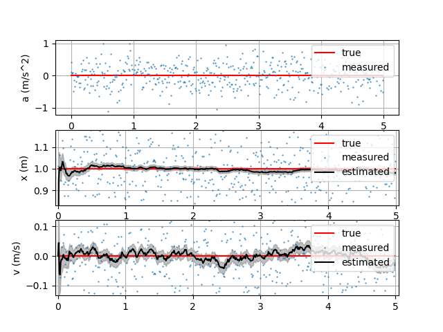
Target is not moving and is fixed at x=1m position. Position error starts large, decreases, and converges to a value. Same with velocity error.
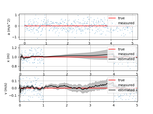
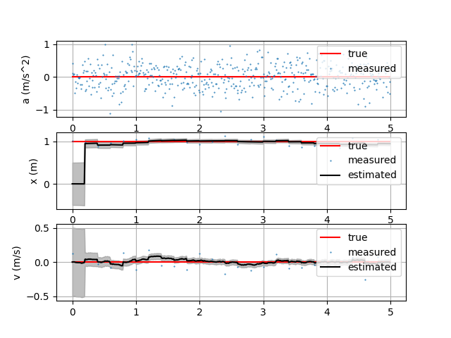
Target is not moving and there is no measurement between 1 to 4 seconds. This is the case when GNSS is temporarily unavailable due to environmnetal factors. Position error increases while there is no measurement. Velocity error also increases while there is no measurement. Both errors diminish once measurement is available.
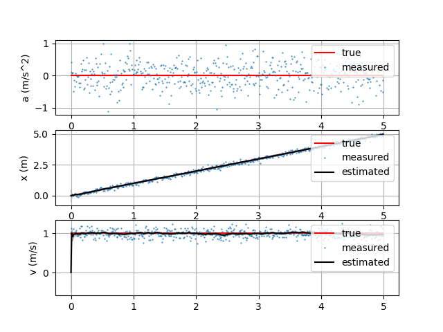
Target moves at a constant speed of 1m/sec. There is no problem tracking.
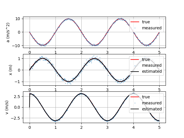
Target moves in a sine wave of 0.5Hz with 1m amplitude. There is no problem tracking thanks to accelerometer input and process noise error.
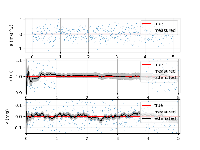
Target is not moving and there is GNSS measurement at 5Hz. This is more realistic because IMU sampling rate is higher than GNSS measurements. There is no problem tracking.
Target is not moving and there is no position measurement between 1 to 4 seconds. This is the case, for example, when using RTK with GNSS: RTK is not fixed (high accuracy position is not available) but GNSS doppler is available (there is velocity measurement). Since we are tracking with only velocity, position error gradually increases over time.
It is assumed that filter.py is placed in the same folder as the below script.
import matplotlib.pyplot as plt
import numpy as np
import filter


random_generator = np.random.default_rng(0)


def plot(t, ground_truth, gnss, a, estimated):
    estimated_x = np.array(estimated['x'])
    estimated_v = np.array(estimated['v'])
    x_std = np.array(estimated['x_std'])
    v_std = np.array(estimated['v_std'])

    fig, axs = plt.subplots(3, 1)

    axs[0].plot(t, ground_truth['a'], color='red', label='true')
    axs[0].plot(t, a, '.', markersize=1, label='measured')
    axs[0].grid(True)
    axs[0].legend(loc='upper right')
    axs[0].set_ylabel('a (m/s^2)')

    axs[1].plot(t, ground_truth['x'], color='red', label='true')
    axs[1].plot(t, gnss['x'], '.', markersize=1, label='measured')
    axs[1].plot(t, estimated_x, color='black', label='estimated')
    axs[1].fill_between(t,
                        estimated_x-x_std,
                        estimated_x+x_std,
                        color='gray', alpha=0.5)
    axs[1].grid(True)
    axs[1].legend(loc='upper right')
    axs[1].set_ylabel('x (m)')

    axs[2].plot(t, ground_truth['v'], color='red', label='true')
    axs[2].plot(t, gnss['v'], '.', markersize=1, label='measured')
    axs[2].plot(t, estimated_v, color='black', label='estimated')
    axs[2].fill_between(t,
                        estimated_v-v_std,
                        estimated_v+v_std,
                        color='gray', alpha=0.5)
    axs[2].grid(True)
    axs[2].legend(loc='upper right')
    axs[2].set_ylabel('v (m/s)')

    plt.show()


def estimate(t, gnss, a):
    N = len(t)
    result = {
        'x'    : [None] * N,
        'v'    : [None] * N,
        'x_std': [None] * N,
        'v_std': [None] * N
    }
    kf = filter.KF()

    result['x'][0] = kf.x[0, 0]
    result['v'][0] = kf.x[1, 0]
    result['x_std'][0] = np.sqrt(kf.P[0, 0])
    result['v_std'][0] = np.sqrt(kf.P[1, 1])
    for i in range(1, N):
        dt = t[i] - t[i-1]
        kf.predict(a[i], dt)
        if ~np.isnan(gnss['x'][i]):
            kf.update_pos(gnss['x'][i], gnss['x_std'][i])
        if ~np.isnan(gnss['v'][i]):
            kf.update_vel(gnss['v'][i], gnss['v_std'][i])
        result['x'][i] = kf.x[0, 0]
        result['v'][i] = kf.x[1, 0]
        result['x_std'][i] = np.sqrt(kf.P[0, 0])
        result['v_std'][i] = np.sqrt(kf.P[1, 1])

    return result


def generate_test1_data():
    # Generate time
    dt = 0.01
    t = np.arange(0, 5, dt)

    # Generate ground truth data
    # Position stationary
    x0 = 1
    ground_truth = {}
    ground_truth['x'] = 0 * t + x0
    ground_truth['v'] = np.gradient(ground_truth['x'], t)
    ground_truth['a'] = np.gradient(ground_truth['v'], t)

    # Generate GNSS sensor data
    stdev = 0.1
    gnss = {
        'x'    : random_generator.normal(ground_truth['x'], stdev),
        'x_std': [stdev] * len(t),
        'v'    : random_generator.normal(ground_truth['v'], stdev),
        'v_std': [stdev] * len(t)
    }

    # Generate accelerometer data
    a = random_generator.normal(ground_truth['a'], 0.35)

    return t, ground_truth, gnss, a


def generate_test2_data():
    # Generate time
    t = np.arange(0, 5, 0.01)

    # Generate ground truth data
    # Position stationary
    x0 = 1
    ground_truth = {}
    ground_truth['x'] = 0 * t + x0
    ground_truth['v'] = np.gradient(ground_truth['x'], t)
    ground_truth['a'] = np.gradient(ground_truth['v'], t)

    # Generate GNSS sensor data
    stdev = 0.1
    gnss = {
        'x'    : random_generator.normal(ground_truth['x'], stdev),
        'x_std': [stdev] * len(t),
        'v'    : random_generator.normal(ground_truth['v'], stdev),
        'v_std': [stdev] * len(t)
    }

    # Remove GNSS data betweeen 1 to 4 seconds
    for i in range(len(t)):
        if t[i] > 1 and t[i] < 4:
            gnss['x'][i], gnss['x_std'][i] = np.nan, np.nan
            gnss['v'][i], gnss['v_std'][i] = np.nan, np.nan

    # Generate accelerometer data
    a = random_generator.normal(ground_truth['a'], 0.35)

    return t, ground_truth, gnss, a


def generate_test3_data():
    # Generate time
    t = np.arange(0, 5, 0.01)

    # Generate ground truth data
    # Position moving at constant velocity
    v = 1
    ground_truth = {}
    ground_truth['x'] = v * t
    ground_truth['v'] = np.gradient(ground_truth['x'], t)
    ground_truth['a'] = np.gradient(ground_truth['v'], t)

    # Generate GNSS sensor data
    stdev = 0.1
    gnss = {
        'x'    : random_generator.normal(ground_truth['x'], stdev),
        'x_std': [stdev] * len(t),
        'v'    : random_generator.normal(ground_truth['v'], stdev),
        'v_std': [stdev] * len(t)
    }

    # Generate accelerometer data
    a = random_generator.normal(ground_truth['a'], 0.35)

    return t, ground_truth, gnss, a


def generate_test4_data():
    # Generate time
    t = np.arange(0, 5, 0.01)

    # Generate ground truth data
    # Position moving in sine wave
    f = 0.5
    ground_truth = {}
    ground_truth['x'] = np.sin(2 * np.pi * f * t)
    ground_truth['v'] = np.gradient(ground_truth['x'], t)
    ground_truth['a'] = np.gradient(ground_truth['v'], t)

    # Generate GNSS sensor data
    stdev = 0.1
    gnss = {
        'x'    : random_generator.normal(ground_truth['x'], stdev),
        'x_std': [stdev] * len(t),
        'v'    : random_generator.normal(ground_truth['v'], stdev),
        'v_std': [stdev] * len(t)
    }

    # Generate accelerometer data
    a = random_generator.normal(ground_truth['a'], 0.35)

    return t, ground_truth, gnss, a


def generate_test5_data():
    # Generate time
    t = np.arange(0, 5, 0.01)

    # Generate ground truth data
    # Position stationary
    x0 = 1
    ground_truth = {}
    ground_truth['x'] = 0 * t + x0
    ground_truth['v'] = np.gradient(ground_truth['x'], t)
    ground_truth['a'] = np.gradient(ground_truth['v'], t)

    # Generate GNSS sensor data
    stdev = 0.1
    gnss = {
        'x'    : random_generator.normal(ground_truth['x'], stdev),
        'x_std': [stdev] * len(t),
        'v'    : random_generator.normal(ground_truth['v'], stdev),
        'v_std': [stdev] * len(t)
    }

    # Make GNSS data sample at 5Hz
    for i in range(len(t)):
        if i % 20 != 0:
            gnss['x'][i], gnss['x_std'][i] = np.nan, np.nan
            gnss['v'][i], gnss['v_std'][i] = np.nan, np.nan

    # Generate accelerometer data
    a = random_generator.normal(ground_truth['a'], 0.35)

    return t, ground_truth, gnss, a


def generate_test6_data():
    # Generate time
    t = np.arange(0, 5, 0.01)

    # Generate ground truth data
    # Position stationary
    x0 = 1
    ground_truth = {}
    ground_truth['x'] = 0 * t + x0
    ground_truth['v'] = np.gradient(ground_truth['x'], t)
    ground_truth['a'] = np.gradient(ground_truth['v'], t)

    # Generate GNSS sensor data
    stdev = 0.1
    gnss = {
        'x'    : random_generator.normal(ground_truth['x'], stdev),
        'x_std': [stdev] * len(t),
        'v'    : random_generator.normal(ground_truth['v'], stdev),
        'v_std': [stdev] * len(t)
    }

    # Remove GNSS position data betweeen 1 to 4 seconds
    for i in range(len(t)):
        if t[i] > 1 and t[i] < 4:
            gnss['x'][i], gnss['x_std'][i] = np.nan, np.nan

    # Generate accelerometer data
    a = random_generator.normal(ground_truth['a'], 0.35)

    return t, ground_truth, gnss, a


# Generate test data
#t, ground_truth, gnss, a = generate_test1_data()
#t, ground_truth, gnss, a = generate_test2_data()
#t, ground_truth, gnss, a = generate_test3_data()
#t, ground_truth, gnss, a = generate_test4_data()
#t, ground_truth, gnss, a = generate_test5_data()
t, ground_truth, gnss, a = generate_test6_data()

# Estimate with Kalman filter
estimated = estimate(t, gnss, a)

# Graph result
plot(t, ground_truth, gnss, a, estimated)