A practical way to find the time response of a system is through simulation. This page discusses four methods to simulate continuous systems:
| Method | Target | |
| 1. | Euler's method | Linear & Nonlinear |
| 2. | Discretization | Linear |
| 3. | lsim() | Linear |
| 4. | ODE solver | Nonlinear |
"Linear" means that the dynamic equations can be written in the state-space form:
"Nonlinear" means that the dynamic equation is in the form:
Examples to simulate trajectory tracking and motor saturation are provided. Methods discussed here can also be extended to include feedforward and state estimation. Example code is written in Python but equivalent functions are available in MATLAB.
This is a quick-and-dirty way to implement a working simulation. It requires no dependence on external libraries so it can be implemented in a variety of languages. The downside is that it is not as accurate as the other methods. It works for both linear and nonlinear systems.
Psuedo code:
x  = x0    // Initial state x(0)
dt = 0.01 // Time step (seconds)

for i = 0 to 99
    t    = i * dt
    xdot = A * x + B * u(t)  // xdot(t) = Ax(t) + Bu(t)
    x    = x + xdot * dt     // x(t+dt) = x(t) + xdot(t)
Example:
Suppose we have a 1-dimensional continuous linear time-invariant system where,

with initial condition,

The analytical solution is,

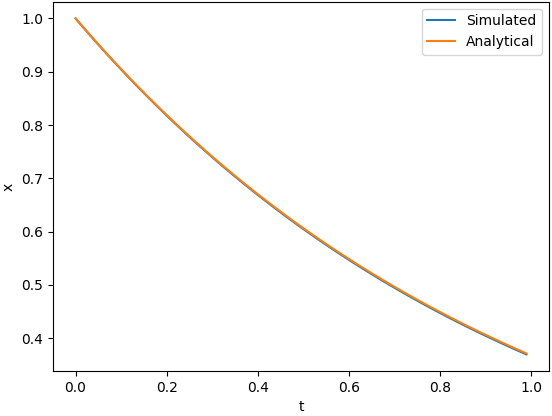
Simulating this with Python:
import matplotlib.pyplot as plt
import numpy as np

dt = 0.01 # Time step
A  = -1   # System matrix
B  = 0    # Input matrix
u  = 0    # Input vector (not used)
x  = 1    # State vector, initial condition: x(0) = 1

ts = []
xs = []

for i in range(100):
    t = i * dt

    ts.append(t)         # t = 0, 0.01, 0.02, ...
    xs.append(x)         # x(t)

    # Update
    xdot = A * x + B * u # xdot(t)
    x += xdot * dt       # x(t+dt)

plt.plot(ts, xs, label='Simulated')
plt.plot(ts, np.exp(-np.array(ts)), label='Analytical')
plt.legend()
plt.xlabel('t')
plt.ylabel('x')
plt.show()
Output:
This method uses the fact that a continuous linear time-invariant system can be discretized analytically to the following form:
Note that the matrices are not the same and ẋ is now x[k+1].
Example:
Suppose we have a continuous linear time-invariant system where,

and we have a control law,
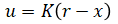
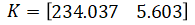
where u is the input vector, K is gain matrix shown below, r is reference state (trajectory), and x is the state vector.
Input, u, is also subject to saturation between -12 and 12. Initial conditions are,

Simulating this with scipy:
import matplotlib.pyplot as plt
import numpy as np
from scipy.signal import StateSpace

def trajectory(t):
    if t < 0.1:
        return np.array([[0.0], [0.0]])
    elif t < 5.1:
        return np.array([[1.524], [0.0]])
    else:
        return np.array([[0.0], [0.0]])

# Time step
dt = 0.005

# Model
A = np.array([[0, 1], [0, -164.209]])
B = np.array([[0], [21.457]])
C = np.array([[1, 0]])
D = np.array([[0]])

# Controller matrices
K = np.array([[234.037, 5.603]])

# State-space model
sysc = StateSpace(A, B, C, D) # Continuous
sysd = sysc.to_discrete(dt)   # Discrete

# Vectors
x = np.asarray(np.zeros((2, 1)))   # State vector 2x1
u = np.asarray(np.zeros((1, 1)))   # Input vector 1x1
y = np.zeros((sysc.C.shape[0], 1)) # Output vector 1x1
r = np.zeros((sysc.A.shape[0], 1)) # Reference vector 2x1

# Time
ts = np.arange(0, 10.2, dt)

# For logging
x_rec = np.zeros((sysd.A.shape[0], 0))
r_rec = np.zeros((sysd.A.shape[0], 0))
u_rec = np.zeros((sysd.B.shape[1], 0))
y_rec = np.zeros((sysd.C.shape[0], 0))

# Run simulation
for t in ts:
    # Update plant
    x = sysd.A @ x + sysd.B @ u
    y = sysd.C @ x + sysd.D @ u

    # Update controller
    r = trajectory(t) # Reference
    u = K @ (r - x)
    u = np.clip(u, -12.0, 12.0) # Saturation

    # Log states for plotting
    x_rec = np.c_[x_rec, x]
    r_rec = np.c_[r_rec, r]
    u_rec = np.c_[u_rec, u]
    y_rec = np.c_[y_rec, y]

fig, axs = plt.subplots(3, 1)
axs[0].set_ylabel('u')
axs[0].plot(ts, np.squeeze(u_rec[0, :]))
axs[1].set_ylabel('x1')
axs[1].plot(ts, np.squeeze(x_rec[0, :]), label='State')
axs[1].plot(ts, np.squeeze(r_rec[0, :]), label='Reference')
axs[1].legend()
axs[2].set_ylabel('x2')
axs[2].plot(ts, np.squeeze(x_rec[1, :]), label='State')
axs[2].plot(ts, np.squeeze(r_rec[1, :]), label='Reference')
axs[2].legend()
axs[2].set_xlabel('t')
plt.show()
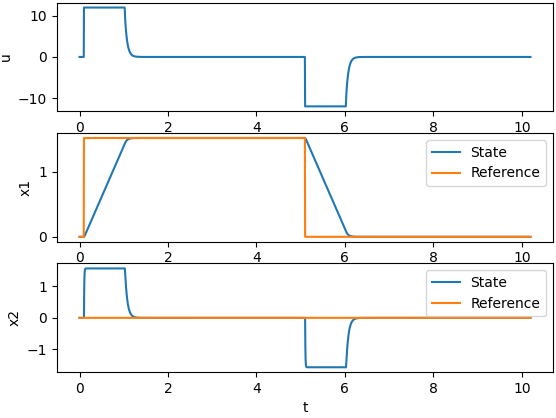
Output (note that u is saturated):
to_discrete() takes dt (time step) as input and returns a discrete version of the system using a method called "zero-order hold." Directly specifying dt in the StateSpace constructor also works. The same can be achieved using Python's control package. MATLAB has c2d function that converts a model from continuous to discrete time.
lsim() is a MATLAB function to simulate linear time-invariant systems. Python's equivalent is scipy.signal.lsim() and control.matlab.lsim() and control.forced_response(). This also uses zero-order hold method by default. It is possible to do feedback control using the fact that,
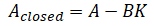
but to do more complex modifications to the input, u (for example to simulate saturation), divide the time into smaller steps and call the simulation function multiple times.
Example:
This is the same example as that of the previous section but uses control.forced_response() instead.
import matplotlib.pyplot as plt
import numpy as np
import control

def trajectory(t):
    if t < 0.1:
        return np.array([[0.0], [0.0]])
    elif t < 5.1:
        return np.array([[1.524], [0.0]])
    else:
        return np.array([[0.0], [0.0]])

# Time step
dt = 0.005

# Model
A = np.array([[0, 1], [0, -164.209]])
B = np.array([[0], [21.457]])
C = np.array([[1, 0]])
D = np.array([[0]])

# Controller matrices
K = np.array([[234.037, 5.603]])

# State-space model
sys = control.StateSpace(A, B, C, D) # Continuous

# Vectors
x = np.asarray(np.zeros((2, 1)))  # State vector 2x1
u = np.asarray(np.zeros((1, 1)))  # Input vector 1x1
y = np.zeros((sys.C.shape[0], 1)) # Output vector 1x1
r = np.zeros((sys.A.shape[0], 1)) # Reference vector 2x1

# Time
ts = np.arange(0, 10.2, dt)

# For logging
x_rec = np.zeros((sys.A.shape[0], 0))
r_rec = np.zeros((sys.A.shape[0], 0))
u_rec = np.zeros((sys.B.shape[1], 0))
y_rec = np.zeros((sys.C.shape[0], 0))

# Run simulation
for t in ts:
    # Update plant
    T = [t, t + dt]
    U = np.c_[u, u]
    X0 = x
    T, y, x = control.forced_response(sys, T, U, X0, return_x=True)
    y = y[-1]
    x = x[:, [-1]]

    # Update controller
    r = trajectory(t) # Reference
    u = K @ (r - x)
    u = np.clip(u, -12.0, 12.0) # Saturation

    # Log states for plotting
    x_rec = np.c_[x_rec, x]
    r_rec = np.c_[r_rec, r]
    u_rec = np.c_[u_rec, u]

fig, axs = plt.subplots(3, 1)
axs[0].set_ylabel('u')
axs[0].plot(ts, np.squeeze(u_rec[0, :]))
axs[1].set_ylabel('x1')
axs[1].plot(ts, np.squeeze(x_rec[0, :]), label='State')
axs[1].plot(ts, np.squeeze(r_rec[0, :]), label='Reference')
axs[1].legend()
axs[2].set_ylabel('x2')
axs[2].plot(ts, np.squeeze(x_rec[1, :]), label='State')
axs[2].plot(ts, np.squeeze(r_rec[1, :]), label='Reference')
axs[2].legend()
axs[2].set_xlabel('t')
plt.show()
Output is the same as that from previous section.
This last approach is for nonlinear systems. For MATLAB use ode45() and for python use scipy.integrate.solve_ivp() or scipy.integrate.odeint(). Both use Runge-Kutta method by default.
Example:
Suppose we have a nonlinear model,
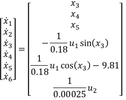
and a controller,
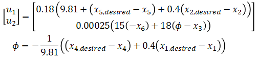
with input saturation and a reference trajectory to track.
This can be simulated using scipy.integrate.solve_ivp() as follows:
from math import sin, cos
from scipy.integrate import solve_ivp
import matplotlib.pyplot as plt

def xdot(t, x):
    # Trajectory (reference)
    if t < 1:
        x_des = [0, 0, 0, 0, 0, 0]
    else:
        x_des = [0.5, 0, 0, 0, 0, 0]

    # Controller
    phi_c = -1/9.81 * ((x_des[3] - x[3]) + 0.4 * (x_des[0] - x[0]))
    u = [0.18 * (9.81 + (x_des[4] - x[4]) + 0.4 * (x_des[1] - x[1])),
         0.00025 * (15 * (-x[5]) + 18 * (phi_c - x[2]))]

    # Saturation
    v1 = 0.5*(u[0] - u[1]/0.086)
    v2 = 0.5*(u[0] + u[1]/0.086)
    v1_clamped = min(max(0, v1), 1.7658)
    v2_clamped = min(max(0, v2), 1.7658)
    u = [v1_clamped + v2_clamped,
         (v2_clamped - v1_clamped) * 0.086]

    # First derivative, xdot
    return [x[3],
            x[4],
            x[5],
            -u[0] * sin(x[2]) / 0.18,
            u[0] * cos(x[2]) / 0.18 - 9.81,
            u[1] / 0.00025]

x0     = [0, 0, 0, 0, 0, 0] # Initial state
t_span = [0, 20]            # Simulation time [from, to]

# Run simulation
sol = solve_ivp(xdot, t_span, x0)

# Plot
fig, axs = plt.subplots(3)
axs[0].set_ylabel('x1')
axs[0].plot(sol.t, sol.y[0])
axs[1].set_ylabel('x2')
axs[1].plot(sol.t, sol.y[1])
axs[2].set_ylabel('x3')
axs[2].plot(sol.t, sol.y[2])
axs[2].set_xlabel('t')
plt.show()
Output:
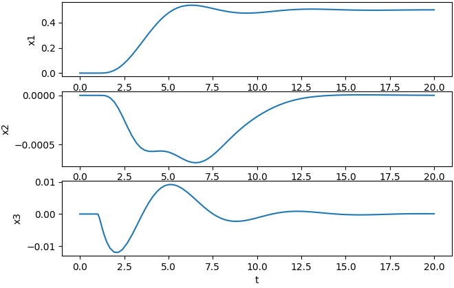
Like lsim(), time can be divided into smaller steps and the integrator function called multiple times. This is useful when the integrator is taking too long to compute or if you need to show some sort of animation in real-time.