PD controller is developed to control a quadrotor in 2-dimensional space.
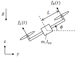
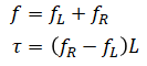
The quadrotor has two inputs: motor thrusts from the left and the right motors. They cause a net force and torque applied to the quadrotor:
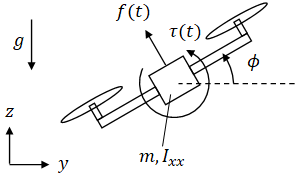
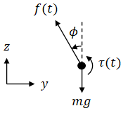
The net force and torque will be used as the two inputs to the quadrotor to simplify subsequent calculations. The new schematic diagram becomes:
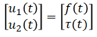
| (input) | f(t) | = | force applied on the quadrotor by the motors | |
| (input) | τ(t) | = | torque applied on the quadrotor by the motors | |
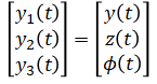
| (output) | y(t) | = | horizontal position | unknown |
| (output) | z(t) | = | vertical position (height) | unknown |
| (output) | Φ(t) | = | tilt (angle) | unknown |
| m | = | mass | ||
| Ixx | = | moment of inertia | ||
| g | = | gravitational acceleration |
3 unknowns so 3 equations are needed.
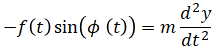
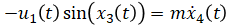
Newton's 2nd law (y-axis):
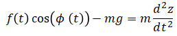
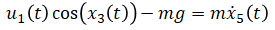
Newton's 2nd law (z-axis):
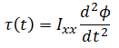
Newton's 2nd law (rotation):
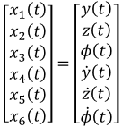
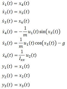
States:

Position and velocity are chosen as state variables because,
State vector:
Input vector:
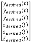
Output vector:
Rewrite (eq. 1) in these new notations:
Rewrite (eq. 2) in these new notations:
Rewrite (eq. 3) in these new notations:
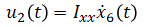
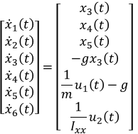
Rearrange equations to express ẋ(t) and y(t) in terms of x(t) and u(t):
Rewrite as matrix:
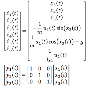
The dynamics model is nonlinear because it is not of the form ẋ=Ax+Bu.
PD controller is designed for linear systems so the dynamics model is first linearized. Model is linearized at the equilibrium point, that is, at hover configuration. At this point, the following is true:
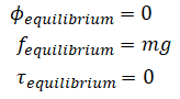
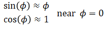
Trigonometric functions can also be linearized at this equilibrium point using first order Taylor approximation:
Using these facts, linearized dynamics model can be written as:
The objective is to design a controller (find the input force and torque functions) which makes the quadrotor track a trajectory (position, velocity, and acceleration as a function of time).
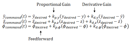
PD controller can be written as,
(eq. 4) can be solved for the inputs:
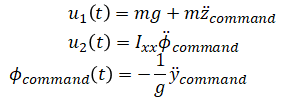
Substitute the PD controller to obtain the control equations:
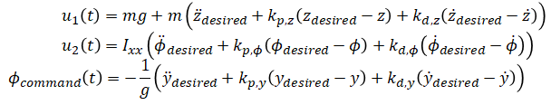
There are still four unresolved variables:

Because Φ cannot be commanded directly, let Φcommand=Φdesired:

The derivatives of Φcommand can be approximated as 0:
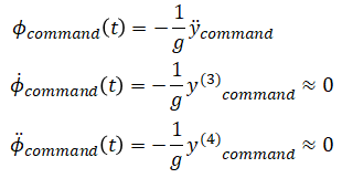
The derivative of Φcommand is proportional to the third derivative of y (jerk in the horizontal direction). The second derivative of Φcommand is proportional to the fourth derivative of y (snap in the horizontal direction). For non-aggressive trajectories with small jerk and snap, these can be approximated as 0.
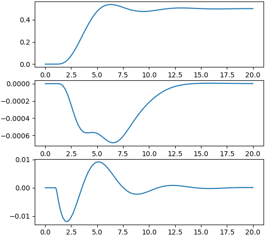
Python code simulation. Quadrotor hovers for 1 second and then tries to reach target position of z=0m and y=0.5.
from math import sin, cos
from scipy.integrate import solve_ivp
import matplotlib.pyplot as plt


# Constants
g     = 9.81    # Gravitational acceleration (m/s^2)
m     = 0.18    # Mass (kg)
Ixx   = 0.00025 # Mass moment of inertia (kg*m^2)
L     = 0.086   # Arm length (m)


# Returns the desired position, velocity, and acceleration at a given time.
# Trajectory is a step (y changes from 0 to 0.5 at t=1)
#
# t     : Time (seconds), scalar
# return: Desired position & velocity & acceleration, y, z, vy, vz, ay, az
def trajectory(t):
    if t < 1:
        y = 0
    else:
        y = 0.5
    z = 0
    vy = 0
    vz = 0
    ay = 0
    az = 0

    return y, z, vy, vz, ay, az


# Returns force and moment to achieve desired state given current state.
# Calculates using PD controller.
#
# x     : Current state, [y, z, phi, vy, vz, phidot]
# y_des : desired y
# z_des : desired z
# vy_des: desired y velocity
# vz_des: desired z velocity
# ay_des: desired y acceleration
# az_des: desired z acceleration
# return: Force and moment to achieve desired state
def controller(x, y_des, z_des, vy_des, vz_des, ay_des, az_des):
    Kp_y   = 0.4
    Kv_y   = 1.0
    Kp_z   = 0.4
    Kv_z   = 1.0
    Kp_phi = 18
    Kv_phi = 15

    phi_c = -1/g * (ay_des + Kv_y * (vy_des - x[3]) + Kp_y * (y_des - x[0]))
    F = m * (g + az_des + Kv_z * (vz_des - x[4]) + Kp_z * (z_des - x[1]))
    M = Ixx * (Kv_phi * (-x[5]) + Kp_phi * (phi_c - x[2]))

    return F, M


# Limit force and moment to prevent saturating the motor
# Clamp F and M such that u1 and u2 are between 0 and 1.7658
#
#    u1      u2
#  _____    _____
#    |________|
#
# F = u1 + u2
# M = (u2 - u1)*L
def clamp(F, M):
    u1 = 0.5*(F - M/L)
    u2 = 0.5*(F + M/L)

    if u1 < 0 or u1 > 1.7658 or u2 < 0 or u2 > 1.7658:
        print(f'motor saturation {u1} {u2}')

    u1_clamped = min(max(0, u1), 1.7658)
    u2_clamped = min(max(0, u2), 1.7658)
    F_clamped = u1_clamped + u2_clamped
    M_clamped = (u2_clamped - u1_clamped) * L

    return F_clamped, M_clamped


# Equation of motion
# dx/dt = f(t, x)
#
# t     : Current time (seconds), scalar
# x     : Current state, [y, z, phi, vy, vz, phidot]
# return: First derivative of state, [vy, vz, phidot, ay, az, phidotdot]
def xdot(t, x):
    y_des, z_des, vy_des, vz_des, ay_des, az_des = trajectory(t)
    F, M = controller(x, y_des, z_des, vy_des, vz_des, ay_des, az_des)
    F_clamped, M_clamped = clamp(F, M)

    # First derivative, xdot = [vy, vz, phidot, ay, az, phidotdot]
    return [x[3],
            x[4],
            x[5],
            -F_clamped * sin(x[2]) / m,
            F_clamped * cos(x[2]) / m - g,
            M_clamped / Ixx]


x0     = [0, 0, 0, 0, 0, 0] # Initial state [y0, z0, phi0, vy0, vz0, phidot0]
t_span = [0, 20]            # Simulation time (seconds) [from, to]


# Solve for the states, x(t) = [y(t), z(t), phi(t), vy(t), vz(t), phidot(t)]
sol = solve_ivp(xdot, t_span, x0)


# Plot
fig, axs = plt.subplots(3)
axs[0].plot(sol.t, sol.y[0]) # y   vs t
axs[1].plot(sol.t, sol.y[1]) # z   vs t
axs[2].plot(sol.t, sol.y[2]) # phi vs t
plt.show()
Result:
Note 1: PID is better when there are disturbances (like wind) and modeling errors (unknown mass) because it makes steady-state error go to zero. In such case, the closed loop system becomes third-order.
Note 2: information on this page is based off of an example in an online course[1]. It is modified and extended with additional information.
[1] Coursera, Robotics: Aerial Robotics